A Technical Decomposition of Project Schedules and Production System Models

Introduction

Project schedules are the universal language of project management. Across industries like construction, engineering, software development, defense, energy, the schedule is the primary tool for communicating planned work, coordinating teams, satisfying stakeholder expectations, and defining what needs to happen and by when.

A useful analogy comes from manufacturing. A demand forecast tells you what you desire to produce in response to some known and estimated market demand, i.e., a production target. It does not describe the factory floor and does not tell you whether your production system can meet that demand, where bottlenecks will form, or how variability will affect output. A schedule operates the same way. It tells you what you desire to complete and by when and provides an indication of how scopes are intended to be sequenced. It does not describe how work is done, where work waits, how resources interact, how variability propagates, or whether the system can deliver what the schedule plans.

The gap between a schedule and a production system model is structural. It is not a matter of schedule quality. A schedule built with exceptional care, subject matter expert (SME) input, detailed activity decomposition, and analyzed using Monte Carlo simulation is still a schedule. Its architecture of activities, durations, dependencies, resource assignments was designed to answer sequencing, coordination, and financial questions: what needs to happen, in what order, by when, and at what planned cost. That architecture was built for a specific purpose. What it can model follows from that design.

This paper decomposes both project schedules and production system models technically and lets the comparison speak. The reader will see the inputs each model requires, the assumptions each model makes and the outputs each model can produce.

Project Schedules

A project schedule is a time-ordered model of planned work. It represents activities along with their estimated durations, logical dependencies, and in some cases the resources required to execute them. Its native output is a timeline describing when each activity is planned to start and finish, and when the project is planned to complete. Everything a schedule produces flows from this structure [1].

Origins

In the early 1910’s, Frederick W. Taylor’s The Principles of Scientific Management (1911) established a “planning department” to be a function separate from execution, staffed by specialists who used time studies to set standard task durations, with a routing system to sequence work [2]. Taylor’s associated concept of “functional foremanship” split planning roles (route clerk, instruction card clerk, time and cost clerk, disciplinarian) from production roles (speed boss, gang boss, repair boss, inspector) [2]. This planning and execution split, and the principle that durations should be measured and standardized rather than estimated, is foundational to how project schedules are constructed today.

Henry Gantt, who worked for Taylor, created the well-known bar chart used in virtually all project scheduling software today. From his own account in Organizing for Work (1919), Gantt’s chart plots tasks on one axis and time on the other, displaying planned work alongside actual progress so that lags become visible at a glance [3]. An early version of this chart was used at the Frankford Arsenal before U.S. entry into World War I in April 1917 and was subsequently extended across the Ordnance Department by Brigadier General William Crozier during the war [3]. This wartime implementation served as the conceptual and operational testing ground for scheduling large-scale public infrastructure. The logistical success during the war directly paved the way for Gantt charts to be adopted by massive mid-century projects like the construction of the Hoover Dam and the Interstate Highway System.

Daniel J. Hauer translated Taylor's scientific-management principles – the separation of planning and doing, standardized methods, and incentive pay – from their manufacturing origins into the context of construction contracting [4]. Building on the planning framework, Hauer applied time-and-motion study directly to construction trades rather than factory tasks, using shovel work as an extended case study in standardizing task methods and durations [4]. He documented a time-schedule practice paired with "graphic progress charts and diagrams," plotting planned work against a curve or line chart with actual progress tracked against the same standard [4]. Hauer also set out supporting systems that surround a schedule in practice: detailed cost-keeping and book-keeping methods for tracking work against budget, a Task-and-Bonus incentive structure for rewarding workmen, and record-keeping systems for organizing the contracting firm and tracking the deployment of plant and equipment across jobs [4].

Years later, in late 1956, DuPont's Integrated Engineering Control Group initiated a survey into using electronic computers to manage the complexity of large engineering projects, with Remington Rand UNIVAC providing technical support through Kelley [5]. The resulting Critical Path Method was applied first to chemical plant construction and subsequently to plant maintenance shutdowns at DuPont's Louisville Works [5]. Its design intent was precise: given a set of activities with known durations and logical dependencies, what is the minimum time to project completion, and which activities determine that time? CPM was engineered to answer that sequencing and coordination question, and its deterministic structure became the architectural foundation of virtually all modern project scheduling tools and practice [1].

PERT was developed concurrently and independently by the U.S. Navy's Special Projects Office for the Polaris Missile Program, introducing probabilistic three-point duration estimates to address uncertainty in activity durations [5, 6]. PERT did not become the basis of standard scheduling practice. CPM's deterministic structure is what took hold. Today, modern scheduling tools support resource loading, cost integration, earned value reporting, and Monte Carlo simulation. The underlying architecture of activities, durations, and dependencies remains unchanged from its origins.

Schedule Core Inputs

A schedule is built from four structural inputs:

1. Activities – discrete chunks of planned work representing the decomposed tasks that together constitute the project scope
2. Durations – the estimated time each activity requires to complete
3. Dependencies – the logical relationships between activities describing which must precede others before work can begin or finish
4. Resources – assigned to activities to represent who or what performs the work

In practice, activities are typically derived from a Work Breakdown Structure (WBS), which decomposes total project scope into discrete, measurable work packages. The WBS is not a structural input to the CPM algorithm itself (CPM requires only activities, durations, and dependencies) but it is the standard decomposition mechanism from which activities are drawn. When a schedule is cost-loaded for performance measurement, the WBS becomes a structural prerequisite, as discussed in the EVA section below [7].

These four inputs constitute the complete structural vocabulary of a schedule. Everything the schedule produces is derived from them. Durations informed by experienced subject matter experts, engineered process data, well-analyzed historical records, or AI models produce schedules that more accurately represent planned work. That quality, however, is a function of the estimation process, meaning it does not change the structural nature of what the schedule models regardless of how detailed the schedule is.

Embedded Assumptions in Schedules

The core inputs carry embedded assumptions that are structural. They are inherent to the CPM architecture, not artifacts of poor schedule development. They are:

Infinite Capacity – Resources are assumed available when the schedule calls for them. The schedule does not model competing demand on shared resources across the system. This assumption is explicit in the original formulation: Kelley & Walker (1959) state that "the basic assumption that underlies the Critical-Path Method, as developed thus far, is that adequate resources are available to implement any computed schedule." Resource-constrained scheduling emerged as a distinct and computationally harder problem class precisely because CPM does not solve it [8, 9]. The practical consequences of this assumption are significant and have been recognized by practitioners for decades. As John Fondahl observed: "Few of even those who claim to be 'CPM experts' fully appreciate the fact that in a resource-restrained schedule the concept of float and quite often the concept of a critical path breaks down. Since almost all construction projects are resource-restrained at least to some extent, this becomes a major source of problems". When resource constraints are present, the critical path calculated by CPM may not reflect the true controlling sequence of work and float values may be misleading indicators of schedule flexibility.

Deterministic Work – A single duration estimate treats each activity as if its outcome is known in advance. Kelley & Walker (1959) distinguish the "deterministic case" from the "non-deterministic case," treating the latter as an extension rather than part of CPM's core structure [10]. Regardless of whether schedules are deterministic or stochastic, activity duration remains the parameter through which variability is absorbed. Probabilistic approaches such as PERT assign distributions to duration estimates, but variability is still expressed as a property of the activity rather than as an emergent behavior of the production system. This distinction matters because system-level variability arising from interaction effects, congestion, and resource contention is not recoverable from activity-level duration distributions alone [11].

Sequential Dependencies – Work either fully blocks or fully releases. Kelley & Walker (1959) explicitly define the condition: "each job in a project is defined so that it is fully completed before any of its successors can begin." Partial handoffs, feedback loops, and rework cycles are not natively represented in CPM logic. Iterative and concurrent work structures require dependency representations that CPM's original arrow-diagram formalism does not support [12, 13]. Precedence Diagramming Method (PDM) introduced lag and lead relationships as a partial extension [10], but rework loops and feedback remain outside the native logic of both CPM and PDM.

Constant Productivity – CPM does not natively model productivity change over time. Duration estimates are static inputs; the method contains no mechanism for productivity to vary as a function of experience accumulation, crew fatigue, congestion, or system state. A skilled estimator can apply learning curve factors to duration estimates for repetitive activities, partially addressing this within the estimation process. However, dynamic productivity change is not a structural parameter of the schedule itself.

Resource Interchangeability – Resources of the same type are treated as equivalent in CPM logic. Differentiation between individual resource performance levels is not a structural feature of the schedule. The resource-constrained project scheduling literature implicitly encodes this assumption by classifying resources by type rather than by individual unit performance [8].

The relationship between EVA measurement rules and schedule construction introduces an additional practical constraint on how schedules are built. Rules of credit, the methods by which earned value is assigned to work packages, require that activities be structured with boundaries that allow meaningful measurement of completion [14]. EVA requirements influence how work packages are defined, how finely activities are decomposed, and what constitutes a measurable completion event. Schedule construction in EVA is therefore shaped by both CPM logic and the measurement system imposed on it [14, 15].

These assumptions define the architectural boundaries within which CPM operates. They are not correctable through better estimating practice or more detailed schedules. Understanding them is a precondition for understanding what schedules can and cannot predict about project behavior.

Native Outputs of Schedules

A schedule's native outputs follow directly from its inputs and architecture. The primary output is a project timeline: planned start and finish dates for every activity and a calculated project completion date [16]. From that timeline the schedule derives its analytical outputs:

Critical Path – the critical path is the longest continuous sequence of dependent activities through the network. It determines the minimum project duration. Any delay to a critical activity extends the project completion date by an equal amount.

Total & Free Float – Total float is the amount of time an activity can be delayed without delaying the project completion date. Free float is the amount of time an activity can be delayed without delaying any successor activity. Activities on the critical path have zero total float

Relationship Types, Lags, and Date Calculations – activities connect through Finish-to-Start, Start-to-Start, Finish-to-Finish, and Start-to-Finish relationships with lags introducing deliberate time delays between them. From these relationships the schedule computes Early Start, Early Finish, Late Start, and Late finish for every activity. The difference between early and late dates produces float and the activities where that difference is zero form the critical path.

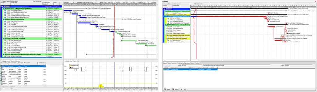
These outputs answer the schedule's native question precisely: when is work planned to happen, which activities control the end date, and where does schedule flexibility exist.

Extensions Practitioners Have Added

Recognizing the limitations of basic CPM scheduling, practitioners have developed several extensions that operate within the schedule framework including, but not limited to:

Monte Carlo simulation propagates uncertainty through the schedule by sampling duration ranges across thousands of iterations, producing a probability distribution of project completion dates rather than a single point estimate [17, 18]. However, most Monte Carlo simulations currently used in the engineering and construction industry follow the approach of using activity durations to absorb all types of variability regardless of source. Regardless of the number of runs and how well durations from past projects are captured, due to the lack of expressiveness in describing the interaction between activities and resources, especially shared resources, the output can be misleading and provides very little room for optimization other than reducing the duration itself or its associated variation.

Resource leveling algorithms resolve resource over-allocation by shifting activities within their float to smooth resource demand across the project timeline, subject to schedule logic constraints [16].

Critical chain project management (CCPM), developed by Goldratt, addresses two structural assumptions in standard CPM: the treatment of work as deterministic and the absence of resource contention. In standard CPM practice, safety time is distributed across individual activity durations. CCPM removes buffers from individual activities and aggregates them into a project buffer at the end of the critical chain and feeding buffers where non-critical paths merge into it. All work not on the critical chain is explicitly subordinated to it. Non-critical-chain work is delayed to its late start, each resource is assigned a single prioritized task at any time, and when a resource completes a task, the chain determines what they work on next. Buffer consumption rates replace date-based milestone tracking as the primary indicator or project health, making remaining contingency visible and actively managed [19].

Duration buffers and schedule contingency represent explicit time reserves added to activity durations or milestone dates to absorb uncertainty [16]. Some call these “fire breaks”.

Beyond these CPM-derived extensions, some practitioners have adopted alternative planning paradigms that address schedule limitations through different means. The Last Planner System (LPS), developed by Glenn Ballard and Greg Howell, shifts planning authority to those closest to the work. Its core mechanism is the distinction between what should be done, what will be done, and what can be done. Crews make weekly commitments only for tasks that are genuinely constraint-free, and performance is tracked through Percent Plan Complete (PPC), a measure of workflow reliability rather than progress against baseline. LPS operates as a production control layer beneath the master schedule, managing short-interval execution through make-ready discipline and constraint removal. It does not model production system behavior quantitatively, but it addresses the gap between a planned sequence and reliable execution that CPM leaves unmanaged [20, 21].

Takt planning applies production rhythm borrowed from manufacturing to construction, dividing scopes into zones and allocating a fixed time interval, the takt time, for each trade to complete its work in each zone before moving to the next [22]. Rather than computing a critical path through dependent activities, takt planning structures the zones, crew sizes, and work packages in a way so that every trade moves through each zone at the same pace [22, 23].

Agile methods emerged from the 2001 Manifesto for Agile Software Development, which prioritized responding to change over following a plan and customer collaboration over contract negotiation [24]. In planning terms, Agile replaces the fixed baseline schedule with short iterative cycles, typically one to four weeks, with scope managed through a prioritized backlog rather than a decomposed WBS, making replanning a structural feature rather than an exception.

These extensions address real limitations within the schedule framework and represent genuine improvements within their respective design intents. However, none turn a schedule into a model of production system behavior.

How Schedules Measure Progress and Performance

Project schedules, when cost-loaded and integrated with a Work Breakdown Structure, form the foundation of Earned Value Analysis (EVA). EVA is the dominant quantitative framework for measuring project progress and forecasting final outcomes [15].

The Work Breakdown Structure decomposes total project scope into discrete, measurable work packages. EVA's effectiveness depends directly on the quality of this decomposition. Well-defined work packages with clear scope boundaries and measurable completion criteria enable accurate performance measurement. The WBS is the structural prerequisite that makes EVA function [7].

EVA measures project performance through three core data points: Budgeted Cost of Work Scheduled, Actual Cost of Work Performed, and Budgeted Cost of Work Performed. From these, five performance metrics are derived: Schedule Variance, Cost Variance, Schedule Performance Index, Cost Performance Index, and Cost Schedule Index.

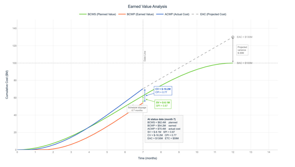
It is worth stating plainly what these metrics measure. Every EVA metric is denominated in cost or a cost-derived ratio. Schedule Variance is expressed in currency, not time. SPI and CPI are ratios of budgeted cost values. The measurement system that dominates project performance reporting is a cost measurement system built on a time-phased schedule baseline [14].

In summary, schedules model the sequence and timing of planned work. When cost-loaded and integrated with a WBS, they produce the performance metrics that dominate project reporting. They answer what is planned, in what order, by who, by when, and at what planned cost.

Production System Models

Production system models are designed to describe and predict how work behaves as it flows through a system of constrained resources over time. Some of the core questions that production system models answer are: What is the capacity of the production system? What is the bottleneck, and does it change? Where does work-in-process accumulate and what is driving it? How does variability appear and propagate through the system? How much WIP should the system contain to maximize throughput and minimize cycle times? In what quantities and frequency should orders be placed for each material? These questions require a different kind of model to answer. The native outputs of a production system model describe system performance: capacity utilization, bottleneck identification, throughput rates, queue lengths, cycle times and their components, and cost and duration distributions. These outputs describe how the system will perform, and therefore, if it meets the demand imposed by the schedule.

Origins

Production system modeling descends from operations research developed during and after World War II and industrial engineering practices formalized through the twentieth century. Queueing theory, pioneered by A.K. Erlang in early telecommunications research and extended by operations researchers including Morse, provides the mathematical foundation, describing the relationships between arrival rates, service rates, utilization, and waiting time [25, 26]. The characterization of a system-limiting resource as a bottleneck has roots in both disciplines. Industrial engineering formalized the problem of allocating work across stations so that no single station limits overall output, known as the assembly line balancing problem, first treated analytically by Salveson in 1955 [27]. Queueing theory established the mathematical characterization independently: the resource with the highest utilization is where queue length grows without bound as arrival rate approaches service rate, making it the determinant of system throughput [25, 28]. Factory Physics later formalized the quantitative laws governing variability, utilization, and cycle time across manufacturing and production environments, establishing that as utilization approaches capacity, cycle time increases nonlinearly, a mathematically derived relationship grounded in queueing theory and empirically validated across production environments [11]. The application of these principles to project-based production environments has been developed and advanced by the Project Production Institute [29]. Together these foundations underpin two distinct modeling approaches used in practice: analytical modeling and discrete event simulation (DES). Each is capable of answering different questions about system behavior depending on the conditions of the system being modeled.

Steady State vs Non-Steady State

Choosing between the modeling approaches requires defining two foundational concepts from queueing theory: system stability and steady state.

A queueing system is stable when the arrival rate of work is strictly less than the service rate of the resource(s) processing it. This is expressed formally as utilization ρ < 1, where ρ = λ / μ [11]. When ρ ≥ 1, arrivals enter the system faster than they can be served and the queue grows without bound. The system never settles, and meaningful long-run performance measures cannot be computed [11]. Stability is therefore a prerequisite condition on the parameters of the system, not on its behavior over time.

Steady state is a condition on the behavior over time, and it is distinct from stability. A stable system that has been running long enough will pass through an initial transient phase such as during startup where the system begins empty and gradually fills. Eventually it reaches statistical equilibrium in which its performance measures: queue lengths, cycle times, utilization, throughput, no longer change with time. At steady state, the system is neither ramping up nor winding down and its structure does not change mid-run. A non-steady state condition exists whenever system behavior changes over time in ways that prevent the equilibrium from being reached or maintained. In project-based production environments, this includes the initial build-up phase where work is entering the system faster than it is leaving, the ramp-down phase as scope completes, and any period where resource counts, routing logic, or demand rates shift mid-execution [30]. Choo notes that in capital construction projects, operations related to engineering, fabrication, transportation, assembly, and commissioning commonly reach a steady state beyond the initial build-up phase, but projects that are too short, too dynamic, or too structurally variable to reach that condition require non-steady state modeling [30]. The distinction matters because the two modeling approaches described below differ precisely in their ability to handle these conditions.

Analytical Modeling vs DES

Production system models are built and run using two complementary methods: analytical modeling and DES. Analytical models apply closed-form mathematical expressions derived from Operations Science to compute system behavior directly. Because the solution is calculated rather than simulated, they execute rapidly and are well-suited to exploring large parameter spaces and optimizing across many variables simultaneously [30]. One central analytical tool for understanding queue behavior is the Kingman equation, which makes visible the three parameters that drive queue time in any production system [31, 13]:

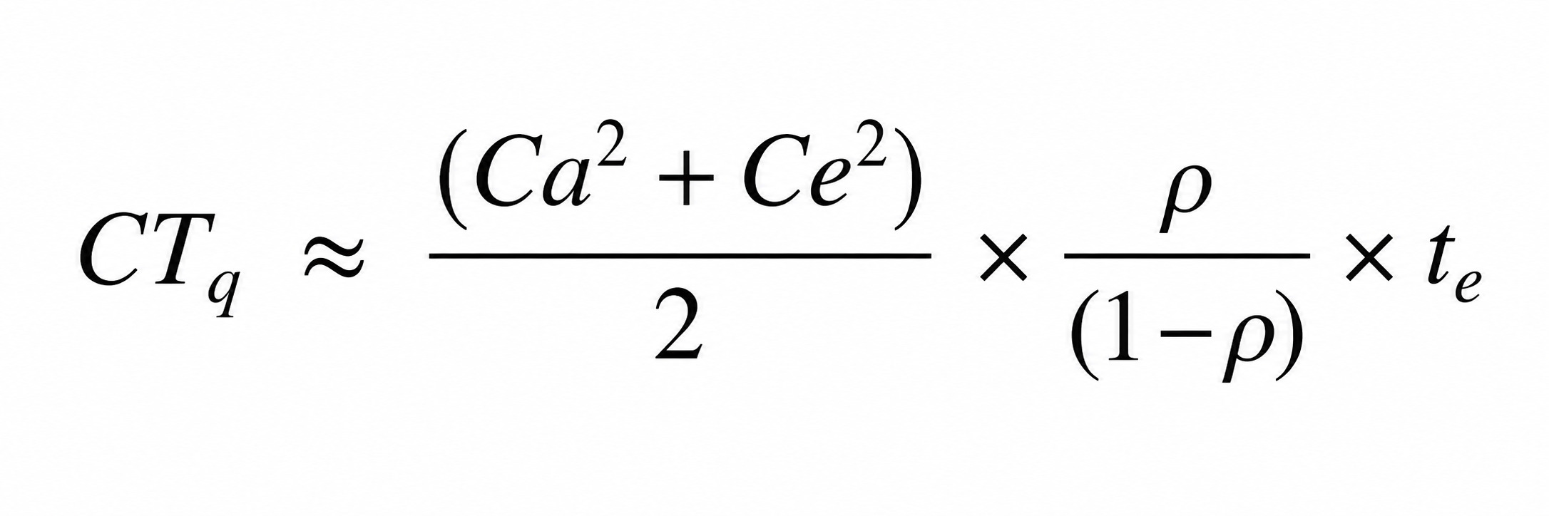
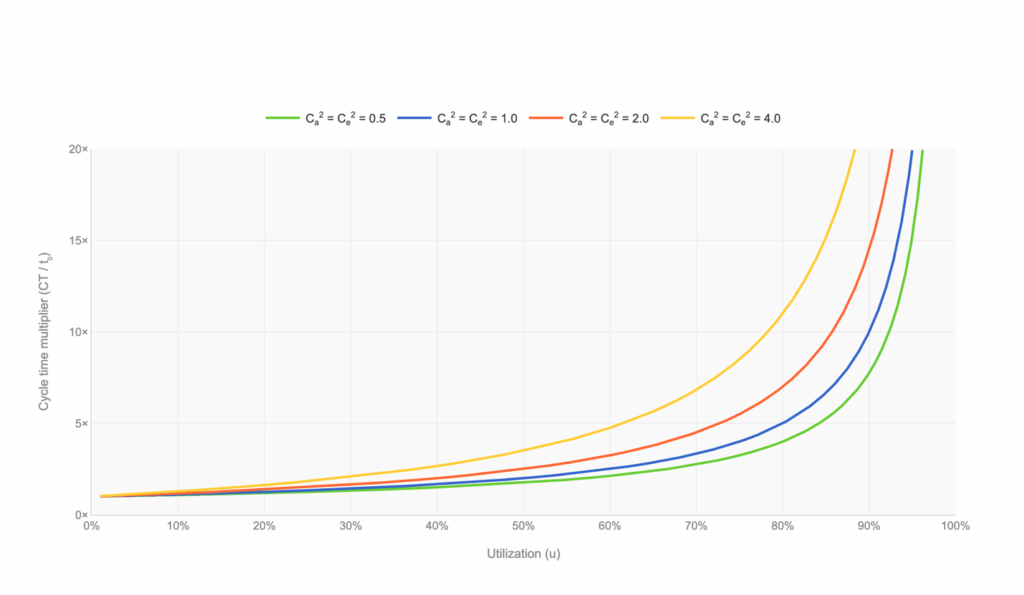
Where Ca² is the squared coefficient of variation of inter-arrival times, Ce² is the squared coefficient of variation of process times, ρ is resource utilization, and is mean effective process time. Queue time is jointly driven by arrival variability and process variability. Queue time increases nonlinearly as utilization approaches 1.0. Analytical modeling reveals minimum WIP required to meet demand, bottleneck resource, cycle time decomposed into its individual components, and the sensitivity of outputs to parameter changes.

Discrete event simulation captures the full dynamic picture of a production system over time that analytical steady-state models cannot capture [30]. Rather than solving for equilibrium, DES models the system by tracking system states at the start and end of each event. Events include taking inputs from inbound queues, holding resources for task duration, and releasing them on completion. Because DES allocates resources only when available, it explicitly models contention between competing work streams at shared resources, transient behavior during ramp-up and ramp-down, and structural changes mid-run that analytical models cannot represent. DES typically takes longer to build and run and optimization across many variables can require large numbers of simulation runs. Integrating analytical modeling as a starting point to identify near-optimal parameters before running DES substantially reduces the effort required to reach a reliable solution [30]. The two approaches are therefore complementary: analytical modeling provides speed and optimization power under steady-state conditions, and DES provides fidelity where system behavior changes over time.

Production System Model Core Inputs

Depending on the type of production system model, the number of inputs can vary. Formulas from Operations Science directly specify exactly which parameters are needed. Each parameter independently shapes how the system behaves.

1. Demand or arrival rates and their variability (Ca²) – the rate at which work enters the system, including the variability in arrival timing that drives queue formation independently of process performance.
2. Bills of materials – the structured enumeration of components, assemblies, and materials required to execute each operation, defining what must be available before work can begin.
3. Operations (process steps) and routing logic – the discrete steps capturing how work transforms as it moves through the system, including sequence, branching paths, feedback loops, and rework cycles.
4. Process times and their variability (Ce²) – how long each operation takes at each resource, expressed as a distribution. Process time variability (Ce²) independently drives queue time and cycle time separate from mean process time.
5. Setup times and their variability – the time required to prepare a resource for a new batch or work type, including the variability in setup time. Setup times consume real resource capacity and interact with batch sizes to affect throughput and cycle time.
6. Resource assignments, quantities, and availability – which resources perform which operations, how many are available, and how often unplanned downtime occurs.
7. Work calendars and their variability – the time patterns governing when resources are available, including shifts, overtime, holidays, and planned downtime.
8. Process and transfer batch sizes – process batch size governs how much work moves through an operation, process, or flow together. Transfer batch size governs how much moves from one step to the next at once. Smaller transfer batches allow downstream operations to begin sooner, directly reducing cycle time.
9. Sequencing rules – the logic that determines which work item is processed next when multiple items are waiting at a resource. Rules like first in first out, last in first out, shortest processing time, and priority-based shape WIP distribution and cycle times without changing total workload.
10. Rework rates and scrap rates and their variability – the fraction of work requiring rework or scrapping. Rework creates feedback loops that increase effective arrival rates at upstream resources, adding to WIP and cycle time. Scrap is lost production requiring additional work be released into the system to meet demand targets.
11. Lead times and their variability – the time between requesting a material and its availability for use. Lead time variability propagates directly into arrival variability at production resources.

These 11 classes of inputs constitute the complete structural vocabulary of a production system model. In specific modeling scenarios, this list may shrink or expand.

Embedded Assumptions in Production System Models

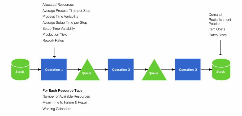
Each type of production system model carries embedded assumptions that are structural to their design. These are the conditions under which each approach produces its most reliable results. Understanding these boundaries enables correct model selection and accurate interpretation of outputs.

Common to both analytical modeling and DES:

Distributional inputs are parameterized from historical performance data or engineering estimates – the quality of those inputs directly determines the reliability of the model.

The model boundary is explicitly defined – work entering and leaving the system crosses a defined boundary; behavior outside that boundary is treated as an external input or not modeled at all.

Resources within a pool are treated as equivalent in capacity – differentiation between individual resource performance levels requires defining separate resource types.

Specific to analytical modeling:

Steady state is assumed – the system's aggregate behavior is stable over the analysis period. However, this does not mean deterministic, i.e., zero variability. Variability in process times, arrival rates, and batch sizes is fully incorporated as input parameters, but dynamic changes in system behavior over time such as ramp-up period where more items are entering the system than leaving require discrete event simulation.

The system structure and inputs are fixed during the analysis period – resource counts, routing logic, batch policies, etc., do not change mid-run.

Variability sources are treated as statistically independent – variability in process times of one operation are independent of another.

Single server approximation – the Kingman equation in its base form approximates behavior for a single server queue (G/G/1). Multi-server queues (G/G/m) can be approximated analytically using the Allen-Cunneen extension. Networks of queues with complex routing, feedback, and non-stationary behavior require either network queueing extensions discrete event simulation.

The assumptions listed above define the operating boundaries of each approach. Where system behavior is stable, analytical modeling delivers speed and mathematical precision. Where behavior is transient or structure changes mid-run, DES is the appropriate approach. The correct model selection depends on the question being asked and the conditions of the system being modeled.

Native Outputs of Production System Models

The native outputs of a production system model are computed directly from the model’s mathematical and simulation structure. Each output describes a specific, measurable property of system behavior.

Capacity – the maximum rate of output a process, routing, or production system can sustain given its resources, calendar, and process design

Throughput – the actual rate of output the system produces under current operating conditions. Throughput is bounded by the bottleneck resource.

Capacity Utilization – the fraction of time that a resource is not idle communicated as an average or as a changing profile over time

Bottleneck Identification – the resource with the highest average capacity utilization over a long period

Optimal WIP Levels – the quantity of work-in-process that maximizes throughput while minimizing cycle time

Optimal Stock Inventory Levels – replenishment policies that minimize cash tied up subject to target fill rate and order frequency

Queue Lengths – the quantity of work waiting at each resource at any point in time. Queue lengths indicate high variability, capacity mismatch, and or large batch sizes

Cycle Times – the total time a unit of work spends in the system from arrival to completion, decomposed into process time, setup time, queue time, batch time, move time, and shift differential time

Predicted Duration – the distribution of total project duration under given input, produced by DES across multiple stochastic runs

Cash Tied Up in Inventory – the monetary value of work-in-process and stock inventory held in the system at any point in time, derived from WIP levels and unit cost

Variability – the statistical dispersion of key outputs, cycle times, throughput rates, queue lengths, across the system and over time, including propagation of variability through the system

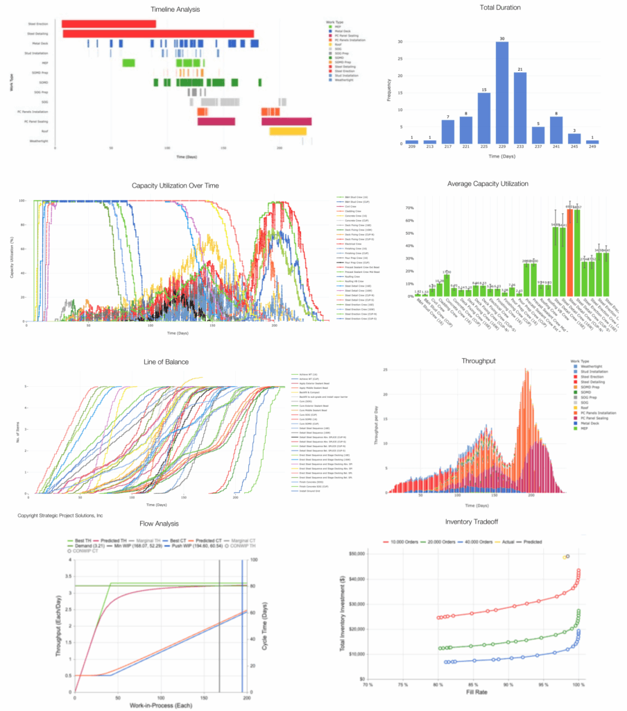
In summary, production system models describe how work behaves as it moves through a system of constrained resources. Their mathematical foundations in Operations Science, provide a rigorous basis for predicting system performance before work begins, identifying areas of production-based risk, and evaluating interventions before they are committed.

Comparison

The preceding decomposition of project schedules and production system models reveals a structural difference in what each model is designed to do, what it requires as input, what it assumes, and what it produces as output. The comparison that follows is a direct consequence of that decomposition.

What The Decomposition Reveals About Project Visibility and Control

The decomposition reveals a structural difference in visibility. A schedule answers whether activities are completing on their planned dates and whether cost is tracking against baseline. The input comparison makes the gap precise: where a schedule requires four inputs, a production system model requires eleven classes. However, their overlap is partial. Schedule durations approximate mean process time (). Resource assignments in a schedule approximate resource availability. The schedule's time dimension combined with bill of quantities data produces a demand rate. Everything else, variability (Ca², Ce²), setup times, batch sizes, sequencing rules, rework rates, lead times, has no equivalent in schedule data and cannot be derived from it.

The Kingman equation makes this gap mathematically explicit. Queue time is a function of Ca², Ce², ρ, and . A schedule contains an approximation of . It structurally cannot contain Ca², Ce², or ρ, as independent parameters. The equation cannot be evaluated from schedule data alone. Additionally, two other phenomena that directly govern production system performance have no representation in schedule inputs: resource interaction effects from competing work streams for shared resources and batching effects from process and transfer batch sizes.

The intuitive optimization target in schedule-driven management is resource efficiency (i.e. keep every resource busy as much as possible). The schedule provides no mechanism to reveal the consequence of this. The Kingman equation establishes that as utilization approaches capacity, cycle time increases nonlinearly [31, 13]. A system running at 90% utilization has dramatically longer queue times than one running at 70% under identical variability conditions. Organizations optimizing for resource efficiency are driving their production systems toward the nonlinear region of the utilization-cycle time curve without a way to see it. Minimizing queue time, which means minimizing the time work spends waiting relative to the time it spends being actively processed, is often the more effective system-level optimization target. This is what some refer to as “flow”. Achieving it requires accepting some resource idle time. That idle time is the capacity buffer that absorbs variability and keeps cycle times stable.

The EVA metrics that dominate project reporting are denominated in cost. While these measurements are important in their own right, none measure throughput, utilization, queue behavior, or cycle time. A project team reading only EVA reports has no visibility into the production systems driving their outcomes.

Conclusion

Schedules earned their formal status because they were adopted as the standard artifact for representing project plans at a time when production system modeling was not yet applied to project environments. The decomposition raises the question of whether the standard artifact list should expand. If production system models provide a qualitatively different and complementary view of project performance, one that is forward-looking, performance based and grounded in the mathematical laws that govern how production systems operate, then the capabilities they enable do not exist without them.

References

1. [1]T. R. Zabelle, G. Fischer, and R. Arbulu, "Schedules vs. project production systems," in 2023 Technical Conference Proceedings, Project Production Institute, 2023.
2. [2]F. W. Taylor, The Principles of Scientific Management. New York, NY, USA: Harper & Brothers, 1911.
3. [3]H. L. Gantt, Organizing for Work. New York, NY, USA: Harcourt, Brace and Howe, 1919.
4. [4]D. J. Hauer, Modern Management Applied to Construction. New York, NY, USA: McGraw-Hill Book Co., 1918.
5. [5]J. E. Kelley and M. R. Walker, "Critical-path planning and scheduling," in Proc. Eastern Joint IRE-AIEE-ACM Computer Conf., Boston, MA, Dec. 1–3, 1959, pp. 160–173.
6. [6]D. G. Malcolm, J. H. Roseboom, C. E. Clark, and W. Fazar, "Application of a technique for research and development program evaluation," Operations Research, vol. 7, no. 5, pp. 646–669, 1959.
7. [7]Project Management Institute, A Guide to the Project Management Body of Knowledge (PMBOK® Guide), 7th ed. Newtown Square, PA: PMI, 2021.
8. [8]J. Blazewicz, J. K. Lenstra, and A. H. G. Rinnooy Kan, "Scheduling subject to resource constraints: Classification and complexity," Discrete Applied Mathematics, vol. 5, no. 1, pp. 11–24, 1983.
9. [9]J. D. Wiest, "A heuristic model for scheduling large projects with limited resources," Management Science, vol. 13, no. 6, pp. B359–B377, 1967.
10. [10]J. J. Moder, C. R. Phillips, and E. W. Davis, Project Management with CPM, PERT and Precedence Diagramming, 3rd ed. New York: Van Nostrand Reinhold, 1983.
11. [11]W. J. Hopp and M. L. Spearman, Factory Physics, 3rd ed. Long Grove, IL: Waveland Press, 2011.
12. [12]T. R. Browning and S. D. Eppinger, "Modeling impacts of process architecture on cost and schedule risk in product development," IEEE Transactions on Engineering Management, vol. 49, no. 4, pp. 428–442, 2002.
13. [13]R. P. Smith and S. D. Eppinger, "Identifying controlling features of engineering design iteration," Management Science, vol. 43, no. 3, pp. 276–293, 1997.
14. [14]Project Management Institute, Practice Standard for Earned Value Management, 2nd ed. Newtown Square, PA: PMI, 2011.
15. [15]ANSI/EIA-748, Earned Value Management Systems Standard. Arlington, VA: Electronic Industries Alliance, 1998 (reaffirmed 2002).
16. [16]Project Management Institute, Practice Standard for Scheduling, 3rd ed. Newtown Square, PA: PMI, 2019.
17. [17]D. Vose, Risk Analysis: A Quantitative Guide, 3rd ed. Chichester, UK: Wiley, 2008.
18. [18]D. Hulett, Practical Schedule Risk Analysis. Farnham, UK: Gower, 2009.
19. [19]E. M. Goldratt, Critical Chain. Croton-on-Hudson, NY: North River Press, 1997.
20. [20]Ballard, G. The Last Planner System of Production Control. Ph.D. Dissertation, University of Birmingham, UK, 2000.
21. [21]Ballard, G. and Howell, G. "Shielding Production: An Essential Step in Production Control." Proceedings of the 6th Annual Conference of the International Group for Lean Construction, Guarujá, Brazil, 1998. (IGLC proceedings paper — not a journal article.)
22. [22]Frandson, A., Berghede, K., and Tommelein, I.D. "Takt Time Planning for Construction of Exterior Cladding." Proceedings IGLC 21, Fortaleza, Brazil, 2013, pp. 527–536.
23. [23]Frandson, A., Berghede, K., and Tommelein, I.D. "Takt-Time Planning and the Last Planner." Proceedings IGLC 22, Oslo, Norway, 2014, pp. 571–580.
24. [24]Beck, K., et al. Manifesto for Agile Software Development. Agile Alliance, 2001. agilemanifesto.org.
25. [25]A. K. Erlang, "The theory of probabilities and telephone conversations," Nyt Tidsskrift for Matematik B, vol. 20, 1909.
26. [26]P. M. Morse, Queues, Inventories and Maintenance. New York: John Wiley & Sons, 1958.
27. [27]M. E. Salveson, "The assembly line balancing problem," Journal of Industrial Engineering, vol. 6, no. 3, pp. 18–25, 1955.
28. [28]L. Kleinrock, Queueing Systems, Volume 1: Theory. New York: Wiley, 1975.
29. [29]Project Production Institute, "Defining 'production system' from an operations science and project production management perspective," Journal of Project Production Management, 2017.
30. [30]H. J. Choo, "More robust, insightful and faster production modeling through the integration of discrete event simulation with analytical modeling," Journal of Project Production Management, Project Production Institute, 2024.
31. [31]J. F. C. Kingman, "The single server queue in heavy traffic," Mathematical Proceedings of the Cambridge Philosophical Society, vol. 57, no. 4, pp. 902–904, 1961.