Beyond Variability: Designing and Controlling Capital Project Production Systems

Introduction

Capital projects are routinely described as uncertain. Schedules slip because of uncertainty, productivity changes because of uncertainty and contingency is consumed because of uncertainty. This language is convenient, but it combines several distinct phenomena into a single category. A permit decision that has not yet been made, an individual crane cycle whose exact duration cannot be predicted, a stable distribution of welding times, a permanent rate mismatch between two crews, and a workforce ramp-up are not the same problem. Treating them as though they were the same encourages the use of the same remedies - more contingency, more detailed planning, or more pressure on execution in an attempt to achieve predictability - even when the underlying production mechanism differs.

Operations Science studies the design and behavior of transformation and flow systems. Its analytical foundations include flow conservation, queue stability, stochastic processes, inventory theory, and production control. These foundations make it possible to distinguish between a knowledge problem, a stochastic process, measurable dispersion, structural differences, and a transient change in operating environment. The distinction matters because a system cannot be improved merely by assigning a label to deviation. It must be diagnosed at the level of the production mechanism.

Consider two concrete crews. If Crew A places 20 m³/hr and Crew B can finish only 15 m³/hr, the queue between them grows at 5 m³/hr even when both rates are perfectly constant. There is no randomness and no within-operation variance. The cause is deterministic rate imbalance. Reverse the rates and the queue does not grow: Crew B is instead starved and has 25% unused capacity. Introduce variation in arrival and finishing times while keeping the average arrival rate below finishing capacity, and a third behavior emerges: a stable but fluctuating queue. That behavior can be approximated using queueing models such as Kingman’s equation [2],[4]. These three cases look superficially similar on a project schedule - one activity feeds another - but they require different countermeasures.

The same issue appears at larger scale. A critical path method (CPM) schedule represents activities, logic, dates, and constraints; it does not by itself represent endogenous queue formation at a shared crane, inspection station, fabrication cell, or commissioning team. Earned Value Management (EVM) can show that earned progress is below planned progress, but conventional Schedule Variance, SV = EV − PV, is expressed in value units and does not identify whether the cause was insufficient capacity, excess WIP, starvation, blocking, rework, or process-time dispersion [9]. Probabilistic schedule-risk analysis can model activity-duration and event risk, but its results do not automatically produce a model of physical production flow. These tools remain useful; the point is that they answer different questions.

This paper answers the following question:

How should Operations Science distinguish uncertainty, randomness, statistical variability, structural heterogeneity, process-rate imbalance, and nonstationarity in capital projects, and what do those distinctions imply for the design and control of buffers?

The paper makes four contributions. First, it provides a terminology and taxonomy that project-delivery practitioners can apply without requiring advanced probability theory. Second, it uses analytical examples to separate deterministic imbalance from stochastic queueing. Third, it interprets the published capacity and time-inventory buffer formulation for capital-project production systems while preserving the distinctions among stock, WIP, queueing time, promised response time, and schedule protection. Fourth, it connects buffer design to Dynamic Risk-based Scheduling (DRS) [3] and Project Production Control [6], including policy optimization, work release, WIP limits, sequence control, capacity adjustment, control-cycle commitments, and environment-change detection.

The framework builds on PPM & Operations Science research to date, including Little’s Law [1], Kingman’s equation [2], Factory Physics [3], general queueing theory [4], CONWIP [5], Dynamic Risk-based Scheduling [3], and Project Production Control [6]. It does not claim that all capital projects are stationary or manufacturing-like. Rather, it identifies project production subsystems and time windows in which particular models are valid, and it makes explicit when transient analysis or discrete event simulation is required.

Conceptual Foundations

Uncertainty: Incomplete Knowledge about Future States

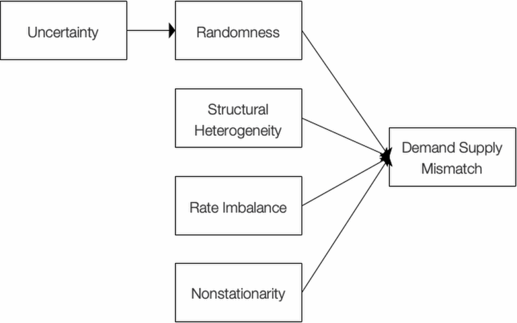
Uncertainty describes the state of knowledge available to a decision-maker. Although much of the production system already exists and is operating in the market before an owner chooses, for instance, air cooling or liquid cooling for a specific data center, the future production system for a given project is not fully defined. Before geotechnical investigation is complete, the foundation solution and production sequence may remain contingent, although the production system for each solution is pretty well known. Before a permit decision, a regulatory pathway may remain unresolved. These are not yet repeated observations from a stable operating process; they are unknown future states or imperfectly known model parameters.

Uncertainty can be epistemic, arising from limited knowledge and therefore potentially reducible through investigation, testing, design development, or expert elicitation. It can also include aleatory elements for which irreducible stochastic models are appropriate. The practical boundary is not always sharp: project teams may use subjective probabilities, Bayesian updating, scenario analysis, or Monte Carlo models even when historical data are sparse. Accordingly, it is too categorical to say that uncertainty is unquantifiable. The more useful distinction is that uncertainty concerns what conditions, design, scope, or production environment will exist, while operational variability concerns behavior within a sufficiently defined environment.

Operational buffers do not eliminate uncertainty. They may protect the project from some consequences of uncertain events - for example, optional specialty capacity, schedule allowance, procurement options, or modular design - but the primary responses also include information acquisition, scenario planning, option design, decision rules, risk treatment, and contractual or commercial allocation. Contractual transfer may reallocate financial consequences; it does not remove physical variability or restore lost production flow.

Randomness: Unpredictability before Realization

Randomness refers to the inability to predict an exact outcome before it occurs, within the chosen model and information set. A truck may arrive at 09:47 today and 10:06 tomorrow. A concrete truck may discharge in 37 minutes on one trip and 42 minutes on the next. A weld repair may or may not be required. Before observation, these outcomes may be modeled as random variables or as events in a stochastic process. After an event occurs, its value is no longer random; it is an observation.

Randomness does not imply disorder or an absence of useful prediction. The next truck arrival may be unknowable to the minute, while hundreds of arrivals exhibit a stable mean, variance, distribution, autocorrelation structure, and time-of-day pattern. For example, a fair six-sided die has an expected value of 3.5. This average does not predict the next roll: the next outcome is random and must be one of the integers from 1 through 6. Indeed, the expected value of 3.5 is not itself a possible individual outcome. Across many rolls, the dispersion of the observed outcomes around 3.5 constitutes statistical variability.Operations Science therefore does not treat randomness as a planning failure. It treats it as a property of the production system model used to represent outcomes and their dependence through time.

Randomness appears throughout capital-project production: welding and inspection durations, crane-cycle times, equipment failures, rework discovery, design-review response times, travel distances, and supplier deliveries. Standard work, automation, mistake-proofing, better logistics, and improved measurement can reduce the observed dispersion and remove assignable causes. They do not guarantee that every future observation becomes exactly predictable.

Statistical Variability: Dispersion in Repeated Observations

Statistical variability is the measurable dispersion of observations around a central tendency. If one thousand cable-tray installations are observed, each realized duration is an observation, and the spread of those durations is statistical variability. It can be described using variance, standard deviation, coefficient of variation (CV), squared coefficient of variation (SCV), quantiles, and a probability distribution.

This definition is narrower and more precise than using variability for every difference in a system. It is the form of variability that enters the VUT representation of queue time through arrival and effective process time SCVs [3]. Statistical variability interacting with finite capacity increases expected waiting, WIP, and cycle time. As utilization approaches one, a stable system becomes increasingly sensitive to a given amount of dispersion.

Randomness describes the unpredictability assigned to outcomes before realization; statistical variability describes differences visible across a set of observations or encoded in the distribution of a process. Randomness is one source of statistical dispersion, but observed dispersion can also contain measurement error, mixed populations, changing conditions, and systematic differences that should be separated rather than pooled.

Structural Heterogeneity and Designed Variation

Capital project work is rarely homogeneous. Pipe spools differ in diameter, material, weld count, support complexity, inspection class, and installation access. Floors may repeat geometrically while differing in embeds, congestion, logistics, or commissioning dependencies. Crew composition and skill mix may differ systematically. Product mix, batch sizes, routings, and work package definitions may change even when execution within each class is deterministic.

These systematic differences are structural heterogeneity. If they are pooled into one distribution without stratification, the reported “variability” may primarily reflect a mixture of unlike work rather than randomness within like-for-like work. That distinction changes the improvement strategy. Standardization, classification, product modularization, routing redesign, work structuring [14], and skill alignment are appropriate responses to structural heterogeneity. A larger generic buffer may conceal the difference without correcting it.

For project practitioners, a useful rule is: before calculating a single mean and standard deviation, ask whether the observations belong to the same production environment. If 150 mm and 600 mm pipe, novice and mature crews, day and night shifts, or uncongested and congested work fronts are combined, the resulting average may not represent any real operating condition.

Rate imbalance: A Deterministic Mismatch of Flow

Rate imbalance occurs when the mean or deterministic output rate of one operation is inconsistent with downstream demand or capability. In a serial system, an upstream rate greater than downstream capacity produces accumulating WIP; an upstream rate below downstream capability produces starvation and idle capacity. This is a flow-balance problem, not necessarily a statistical-variance problem.

The example of Crew A producing three units per minute for Crew B, which can process five units per minute, contains a difference between rates but zero variance in each rate. It is therefore clearer to call the condition rate imbalance or capacity mismatch rather than statistical variability. Crew B is utilized at 3/5 = 0.60 and is starved for 40% of its potential time if no other work is available. Conversely, if Crew A produces five and Crew B can process three, WIP grows at two units per minute, and no finite steady-state queue exists.

This distinction corrects an important conceptual overreach. The statement “variability is the measurable dispersion produced by many random events” is valid as a definition of statistical variability, but it cannot serve as a universal explanation of every flow mismatch. A production system can perform poorly with zero randomness and zero variance.

Nonstationarity: Operating Characteristics that Change through Time

Nonstationarity exists when a relevant mean, variance, distribution, routing, capacity, demand rate, or dependency structure changes through time. Mobilization, learning curves, workforce ramp-up and ramp-down, design maturation, phase transitions, weather seasons, commissioning discovery, and owner priority changes all produce transient environments in capital projects.

For example, a commissioning system may test five subsystems in week one, eighteen in week two, and forty-two in week three while specialist resources and defect discovery also change. A single “average weekly rate” over the three weeks is arithmetically available, but may have little operational meaning. Static equilibrium formulas can obscure the timing of overload and the depletion of buffers.

Nonstationarity should not be confused with high variance. A perfectly smooth capacity ramp is deterministic, but nonstationary. A stationary process can have high variance while retaining stable distributional properties. The analytical consequence is that capacity, arrival rate, WIP, and buffer requirements may need to be represented as functions of time rather than constants.

PHENOMENON	DESCRIPTION	EXAMPLES	SOLUTIONS
Uncertainty	Incomplete knowledge about a future state or parameter	Cooling concept, permit outcome, subsurface condition	Information, scenarios, options, decision rules, risk treatment
Randomness	Unpredictability of an outcome before realization	Next truck arrival or crane-cycle duration	Probability model, standardization, robust design
Statistical variability	Dispersion among like-for-like repeated observations	Range of inspection or installation times	Reduce assignable causes; capacity, WIP/stock, and time protection
Structural heterogeneity	Systematic difference in product, routing, work content, or resource	Different spool classes, crews, shifts, or access zones	Stratification, standardization, modularization, routing and work package redesign
Rate imbalance	Persistent difference between offered load and effective capability	20 m³/hr released to 15 m³/hr finishing	Balance rates, control release, add capacity, redesign, make bottlenecks first, not last, CONWIP
Nonstationarity	Mean, variance, capacity, demand, or routing changes through time	Mobilization, learning, ramp-up, commissioning	Segmentation, cumulative flow, dynamic control, simulation

Table 1. Comparison between Various Sources of Mismatch Between Demand and Supply

From Sources of Mismatch to Flow Consequences

The most general causal concept is not randomness; it is mismatch through time between demand and effective capability. Randomness, structural heterogeneity, rate imbalance, failures, rework, batching, sequencing, and transient change are different sources of that mismatch. Their effects appear as queues, WIP, waiting, stockouts, idle capacity, starvation, blocking, congestion, lost throughput, and unreliable delivery.

Demand and capability must be defined at the same system boundary and in the same units. A crew nominally capable of 20 m³/hr does not provide that capability if access, inspection release, concrete supply, equipment availability, or downstream finishing constraints reduce effective production. Similarly, “demand” may mean customer consumption, authorized work release, upstream output, or a milestone requirement. Confusing these levels creates false utilization estimates.

In a serial production system, five mechanisms deserve separate attention:

1. Starvation: A resource is ready, but lacks released, prerequisite-complete input. The immediate symptom is low utilization; the cause may be insufficient upstream rate, unreliable release, missing information, or excessive batch synchronization.
2. Blocking: A resource cannot release completed work because downstream space, approval, or capacity is unavailable. The blocked resource may appear busy yet produce no usable throughput.
3. Queueing: Released work waits for a finite-capacity resource. In a stable stochastic system, queue length fluctuates around a finite long-run mean. In an overloaded system, it trends upward without bound until the operating environment changes.
4. Rework and recirculation: Work returns to an earlier operation or consumes additional effective process time. Rework both adds load and increases effective-process-time variability.
5. Coordination loss: Shared resources, batch transfers, shift boundaries, access constraints, and priority changes cause effective capability to fall below nominal capability.

These mechanisms can coexist within and across project production systems. A crane may be starved in the morning because lifts are not ready, then become a bottleneck in the afternoon when multiple trades release batches simultaneously. The daily utilization number may look acceptable while both waiting and idle time are high. The production response is not simply to maximize utilization. It is to design release, capacity, sequence, and buffers so the bottleneck and customer-facing flow are protected economically.

The conduit-installation narrative illustrates propagation. An estimate may assign four hours to each installation. In execution, some installations require 3.6 hours and others 4.8 hours; some wait for inspection, materials, access, or a shared lift. If unlike work is mixed, structural heterogeneity inflates the apparent distribution. If arrival and process times fluctuate within a stable environment, statistical variability produces queues. If released conduit work persistently exceeds inspection capacity, deterministic or mean rate imbalance causes backlog growth. If crews are learning or design releases accelerate, the system is nonstationary. Calling all four conditions “uncertainty” prevents a precise diagnosis.

Analytical Foundations

Flow balance and queue stability

Let λ denote the average effective arrival rate to an operation and μ its average effective service rate, expressed in consistent flow units per unit time. For a single-server representation, utilization is:

ρ = λ / μ = λtₑ

A necessary condition for a finite steady-state queue is ρ < 1. If ρ ≥ 1 over the relevant long-run environment, arrivals are not cleared as fast as they enter. When λ > μ and both rates are constant, backlog grows linearly:

Q(t) = Q(0) + (λ − μ)t, for λ > μ

where Q(0) is initial backlog. This is a deterministic conservation statement; it does not require a probability model. When λ = μ with perfectly synchronized deterministic arrivals and service, a zero queue is possible, but the system has no capacity protection. Any disruption, batch release, or timing error can create a queue that cannot be recovered without a subsequent period of μ > λ.

The term capacity buffer therefore needs a precise reference. It can be expressed as an absolute rate margin, Bc = μ − λ, or a relative margin, 1 − ρ. Neither is automatically “good” or “waste.” The appropriate margin depends on variability, response-time requirements, cost, criticality, flexibility, and the consequences of backlog or starvation.

Kingman’s approximation and the VUT relationship

For a stable single-server queue where both customer arrival times and service times follow independent general probability distributions (G/G/1), the commonly used Kingman or VUT approximation for expected queue time is:

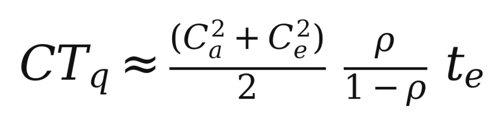
where CTq is expected queue time, Ca² is the SCV of interarrival times, Ce² is the SCV of effective process times, ρ is utilization, and te = 1/μ is the mean effective process time [2, 3, 4]. The equation separates three drivers: variability, utilization, and time. It shows why the same dispersion is far more damaging when utilization is high.

Several boundaries are essential. The approximation assumes a stable, approximately stationary single-server or appropriately aggregated work center representation, utilization below one, finite relevant moments, consistent units, and a queueing discipline for which the approximation is reasonable. It is most accurate for “heavy traffic” which means for utilizations that are above 0.65 or so. Also, it is exact for Poisson arrivals when C_a² = 1 which is a good representation of random arrivals from a large calling population. It does not calculate the waiting time of a permanently growing queue. Substituting ρ > 1 produces a negative denominator and a nonsensical result because the assumptions have been violated, not because waiting time is negative.

The effective process time must include more than touch time when failures, setups, rework, and interruptions consume capacity. If a nominal finishing rate is 20 m³/hr but access loss and equipment downtime reduce the effective rate to 16 m³/hr, μ = 20 overstates the capacity available to clear the queue. Likewise, arrival variability should be measured at the boundary of the analyzed operation, not inferred casually from the variability of upstream processing.

Kingman’s formula is diagnostic, not a universal project-duration formula. It is most useful for repetitive or quasi-repetitive work centers such as fabrication cells, testing stations, inspection processes, logistics gates, and standardized installation systems. Networks with multiple servers, finite buffers, priority classes, blocking, batch transfers, rework loops, and shared resources may require other approximations or discrete-event simulation [4],[11].

Little’s Law

Little’s Law relates long-run averages in a conserved flow system:

L = λW or, in production notation, WIP = TH × CT

In production notation, L is average WIP, λ is average throughput or effective arrival rate in a stable system, and W is average cycle time. Little’s original proof states conditions involving finite means and stationary processes [1]. Later treatments emphasize that the relationship is broad when the system boundary, population, and averaging conventions are consistently defined [12].

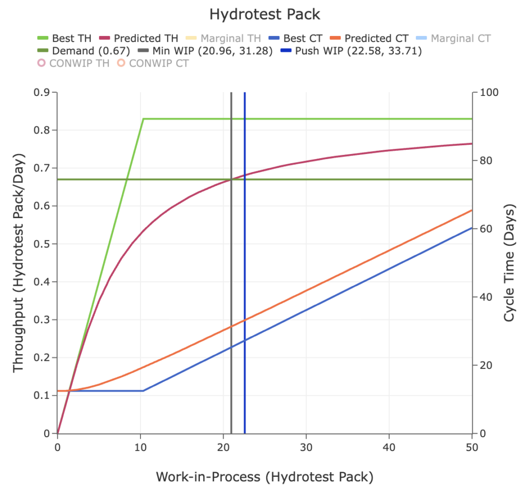
Little’s Law does not mean inventory and time are the same physical quantity. WIP is measured in units, cycle time in time, and throughput in units per time. The variables are linked dimensionally and operationally. At a given throughput, increasing WIP implies proportionally longer cycle times in the near future. The law also does not identify causality: increasing WIP does not necessarily increase throughput, and reducing WIP below the level needed to prevent starvation can reduce throughput (Figure 2).

Cumulative-flow analysis in transient systems

For nonstationary systems, cumulative flow provides a direct representation. Let A(t) be cumulative arrivals or releases and D(t) cumulative departures or completions. Then backlog is:

Q(t) = Q(0) + A(t) − D(t)

Vertical separation between cumulative curves represents units of WIP at a time; horizontal separation represents the elapsed time experienced by a unit, subject to the queue discipline and matching convention. This geometry is the transient counterpart to the long-run relationship embodied in Little’s Law. It makes ramp-up, overload intervals, recovery periods, and buffer consumption visible without assuming constant λ or μ.

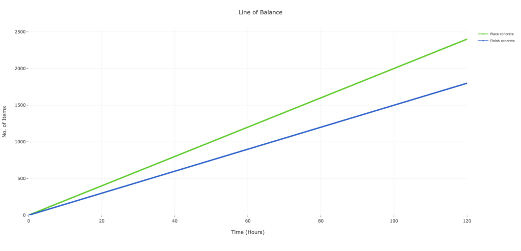
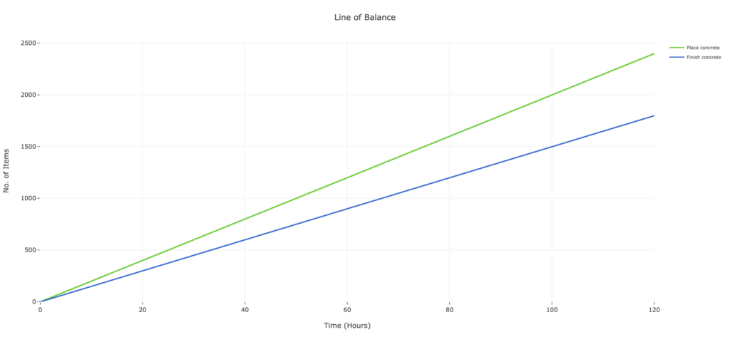
For the concrete example with constant rates 20 and 15 m³/hr, A(t) and D(t) are straight lines whose vertical separation grows at 5 m³/hr (Figure 3). For a workforce ramp-up, the slope of D(t) changes over time. A capacity intervention is visible as an increase in departure slope; a release-control intervention is visible as a reduction or smoothing of arrival slope (Figure 4). A capacity intervention does not always represent adding more resources.

Analytical Model Selection

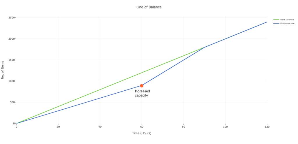
No single formula should be applied simply because data exists. To ensure effective modeling is achieved for specific conditions, the following table provides a framework to conduct a diagnosis:

OBSERVED CONDITION	INITIAL QUESTION	SUITABLE MODEL
Unknown future production environment	What production system, scenario, or set of operating conditions may exist?	Decision analysis, scenario analysis, Bayesian updating and project-risk analysis
Constant deterministic rates	Is flow conserved, and are average demand and effective capability balanced?	Flow conservation equations and cumulative flow analysis
Stable stochastic single work center	Is ρ < 1 and are arrival and effective-process-time distributions approximately stationary?	Kingman/VUT or another queueing model appropriate to the work-center configuration
Stable conserved flow	Are the system boundary, flow unit, throughput and averaging period consistently defined?	Little’s Law, supported by flow-balance and boundary-consistency checks
Ramping or production environment change	How do arrivals, capacity, WIP, stock and completions evolve through time?	Time-varying cumulative-flow analysis, transient queueing models and simulation
Network with shared resources, rework, blocking, priority	Which interactions and policies dominate system performance?	Discrete-event simulation, design of experiments and sensitivity analysis
Production system requiring recurring prediction and control	What is the current system state, how does it differ from expected behavior, and which feasible control action should be taken next?	Production-system digital twin combining state estimation, calibrated analytical or simulation models, DRS policy evaluation and Project Production Control feedback

Table 2. Selection and Operationalization of Operations Science Models

A digital twin is not a substitute for the analytical methods listed above. It synchronizes one or more fit-for-purpose models with the operating production system at a decision-relevant cadence. Its purpose is to estimate current state, diagnose deviations, predict short-horizon behavior, evaluate candidate DRS policies and support Project Production Control decisions. A one-time simulation or a dashboard displaying current values is not, by itself, a digital twin .

Examples of Two-Operation Cases

The following cases use the same boundary: Crew A releases concrete for Crew B to finish. Rates are expressed in m³/hr. The examples abstract from spatial continuity and concrete-setting constraints to isolate the flow mathematics; actual concrete operations require additional engineering constraints.

Case A: Deterministic and Balanced

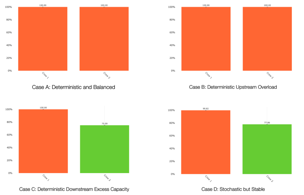
Assume rA = rB = 20 and perfectly synchronized unit flow. Interarrival and process times are deterministic, so Ca² = Ce² = 0. In the idealized model there is no queue and no starvation. Kingman’s expression gives CTq = 0 because the variability term is zero.

This result must not be misread as a robust design because there is always variability in reality. Moreover, utilization is ρ = 1, leaving no recovery capacity. A single delay creates a backlog that cannot be reduced while the rates remain equal. In finite-horizon project work, startup synchronization, shift boundaries, batch transfers, and interruptions make a zero-margin design fragile even when nominal averages are balanced.

Case B: Deterministic Upstream Overload

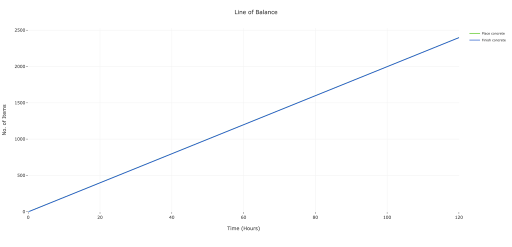
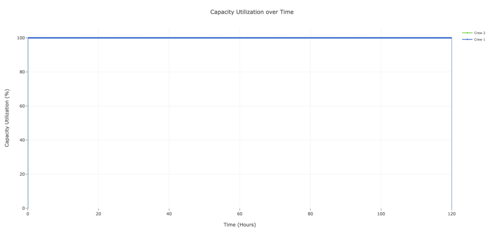
Assume Crew A places at exactly 20 m³/hr and Crew B finishes at exactly 15 m³/hr. The variance of each rate is zero. Downstream utilization calculated from the offered load is:

ρ = 20 / 15 = 1.333 > 1

Because ρ > 1, the system has no finite steady-state queue. With Q(0) = 0:

Q(t) = (20 − 15)t = 5t; Q(4) = 20 m³

After four hours, Q(4) = 20 m³. The approximate workload represented by that backlog at Crew B’s rate is Q/μ = 20/15 = 1.33 hours. A unit entering at the tail at that instant would face approximately this much work ahead under a fluid first-in, first-out interpretation, excluding its own processing and future priority changes.

Kingman’s formula is inapplicable. Entering ρ = 1.333 would yield ρ/(1 − ρ) = −4, an unmistakable assumption failure. The appropriate responses are to reduce release or upstream rate, increase downstream effective capacity, redesign the method, split or resequence work, or deliberately accept and bound the accumulating WIP for a finite interval. Adding a generic “variability buffer” without correcting the mean imbalance cannot produce long-run stability.

Case C: Deterministic Downstream Excess Capacity

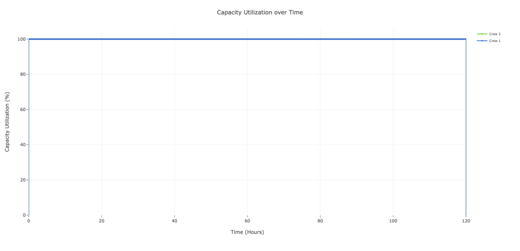
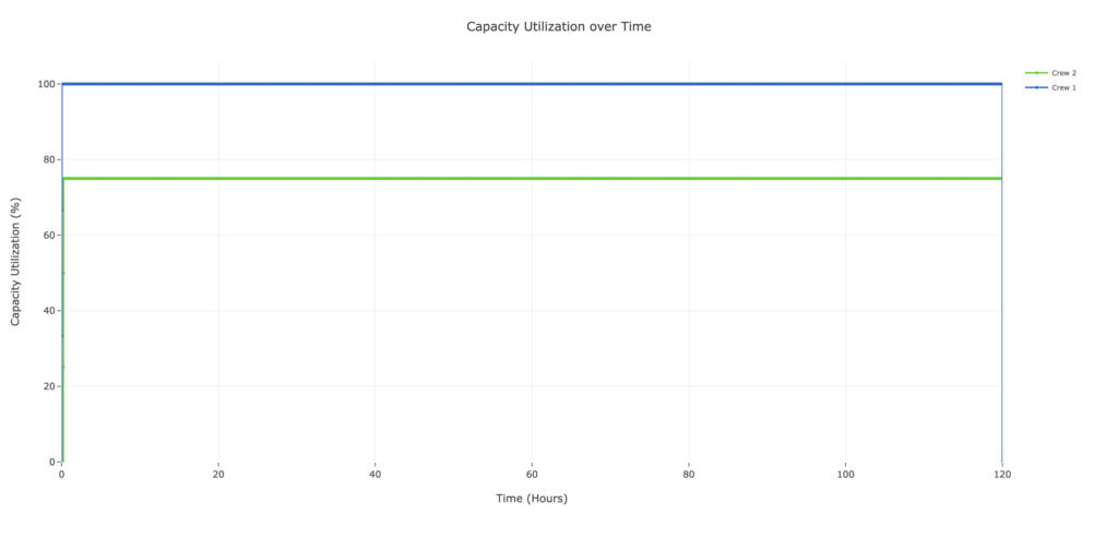
Reverse the rates: Crew A places exactly 15 m³/hr and Crew B can finish exactly 20 m³/hr. Utilization is ρ = 15/20 = 0.75. With deterministic arrivals and service, Ca² = Ce² = 0, so Kingman gives:

Inventory does not grow forever; in the ideal fluid model there is no variability-induced queue. Crew B instead has 5 m³/hr of unused capability, equivalent to 25% of nominal capacity. The unused capacity may be economically undesirable, or it may be an intentional capacity buffer that protects completion flow when arrivals fluctuate. Its value depends on the cost of capacity relative to the cost of waiting, stockout, or milestone delay.

This case demonstrates why “different rates” should not automatically be called statistical variability. The operation is imbalanced, but the flow consequence is starvation rather than congestion.

Case D: Stochastic but Stable

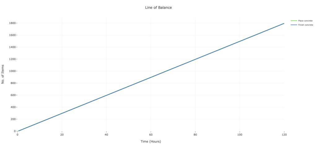
Assume λ = 15 m³/hr, μ = 20 m³/hr, Ca² = 1, and Ce² = 1. Mean effective process time is te = 1/20 hr = 0.05 hr, and ρ = 0.75. Kingman’s equation gives:

The expected queue time is approximately 0.15 hour, or 9 minutes. Expected total cycle time at the work center is CT = CTq + te = 0.20 hour, or 12 minutes per modeled flow unit. Using Little’s Law for the queue, WIPq ≈ TH x CTq = 15 × 0.15 = 2.25 modeled units. The numerical interpretation depends on how a “unit” of concrete flow is defined; a continuous-fluid operation may be better represented with smaller transfer batches or a process-specific model.

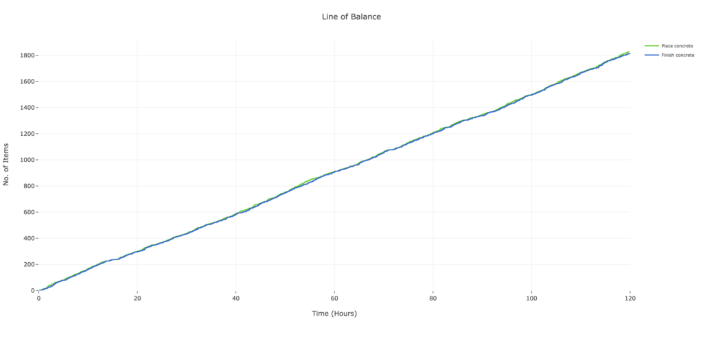
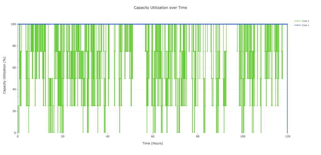
Cases C and D have the same average utilization, yet one has zero queue time in the idealized deterministic model, and the other has positive expected waiting. Case B has zero variance but an unbounded queue. These comparisons isolate the mechanisms that project teams often mix up.

Buffers: Types, Relationships and Project Interpretation

Why Buffers Exist

Transformation and demand cannot generally be synchronized at every instant. If there is a mismatch between demand and supply, and there always is, it will have to be buffered. If there is sufficient completed inventory of work (inventory buffer), the consumer won’t have to wait. If there is not enough, the consumer will have to wait (time buffer). If there is enough capacity (capacity buffer), there is no need for a large stock, and the consumer won’t have to wait long. Since it is impossible to have a stock of finished services, the synchronicity for services must be absorbed by capacity or time buffers.

Buffer Types and Relationships

This specific relationship has been described as follows: if there is variability, it will be absorbed by a combination of the three types of buffers, capacity, inventory, and time [3]. If one of the buffers gets reduced, whether intentionally (inventory through just-in-time initiative, capacity through productivity improvement program, etc.), or unintentionally (number of crew underestimated, not enough inventory to keep the crew busy, etc.), the use of one or both of the other two will increase. It’s simple and logical, but when it is examined using strict definitions and relationships from Operations Science, it leaves a few ambiguities.

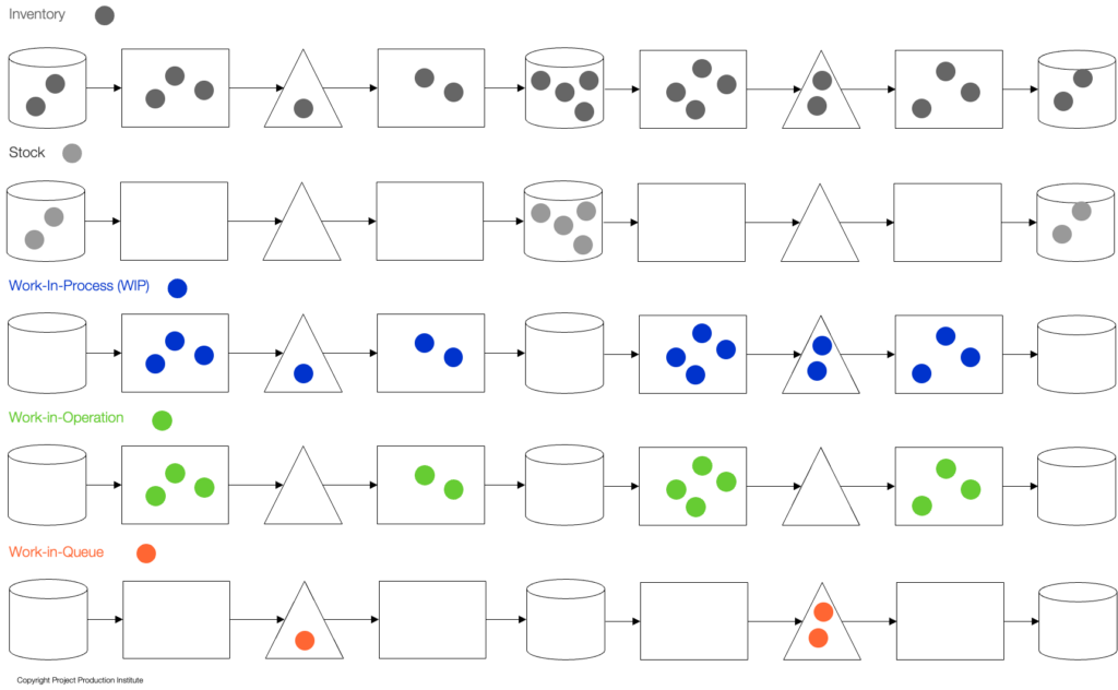
The first is the definition of “inventory”. If we examine the status of inventory throughout a production process, it becomes evident that inventory can take many forms. Inventory that serves as raw material, inventory that is actively being worked on, inventory that is waiting to be worked on between operations, inventory that is completed (a.k.a. finished goods inventory) (Figure 15). However, academic and industry literature and solutions refer to inventory to mean various things.

CONTEXT	TYPICAL USE	INCLUDES
Financial accounting [15]	Current asset reported as inventory	Raw materials, WIP and finished goods, usually measured by monetary value
Retail [16]	Merchandise inventory	Goods held for sale - essentially stock
Warehousing/ERP [17]	Inventory available at a location	Physical on-hand stock
Queueing/flow analysis [12]	Number of entities in the system	WIP, including entities waiting and being processed
Inventory-control theory [18]	Stock governed by replenishment policies	On-hand, on-order, backorders, percent filled from stock, depending on the measure
Construction management [19, 20]	Materials stored onsite or offsite	Uninstalled material stock
Project Production Management [21]	Stock and WIP	Raw materials, WIP and finished goods

Table 3. Various Uses of the Term "Inventory" [12, 15, 16, 17, 18, 19, 20]

However, Little’s Law states Work-In-Process = Throughput x Cycle Time. This indicates WIP is “visible” cycle time. That makes the trade-off between the three types of buffers a bit awkward. Since “inventory” buffer specifically refers to work already completed before demand occurs, it can be concluded that it specifically refers to the “stock” form of inventory. Therefore, a more accurate representation of the three types of buffers is as follows.

The latest update retains capacity, inventory (stock), and time as practical buffering options, but makes a more precise analytical distinction: a target inventory (stock) policy trades inventory against stockouts or backorder time, so inventory and time are “not two buffers” but one time-inventory buffer [13]. In other words, production systems exhibit three observable buffering manifestations - capacity, inventory (stock), and time - but Operations Science combines inventory (stock) and time into one decision because they are jointly determined by the inventory and service policy.

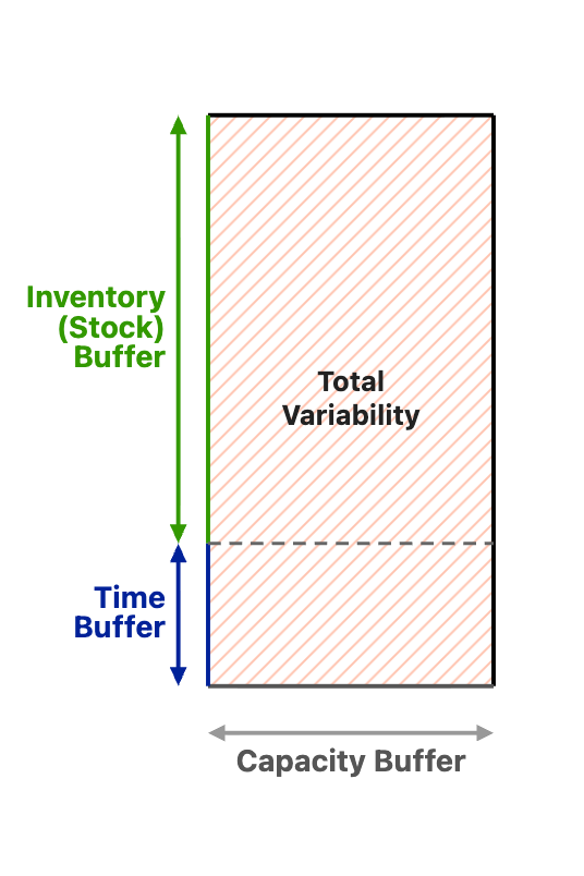
For project delivery, the physical principle should be applied after diagnosis. Buffers can absorb stochastic variation, transient change, batching, and coordination loss, and they can temporarily contain the consequences of deterministic imbalance. They do not make a permanently overloaded system stable, and they should not substitute for rate correction or process redesign.

The definitions and examples are as follows:

• Capacity buffer: effective capability available above the expected offered load over a stated interval. Examples include spare crew capacity, an additional testing team, flexible overtime, redundant equipment, or cross-trained resources.
• Inventory (Stock) manifestation of the time-inventory buffer: units positioned between production and demand. Examples include fabricated modules awaiting installation, released work before inspection, spare materials, finished spools, or completed rooms available for downstream commissioning.
• Time manifestation of the time-inventory buffer: allowable delay between request and fulfillment, planned protection before a milestone, delivery lead-time allowance, or customer tolerance for waiting.

These forms are operationally different. Capacity carries labor, equipment, and opportunity cost. WIP occupies space, hides defects, lengthens feedback, and ties up cash. Finished stock ties up cash and risks damage and obsolescence. Time protection (e.g., long lead times) can delay revenue or reduce responsiveness. Buffer selection is therefore an economic design decision rather than a universal instruction to maximize or minimize one form.

Finally, one must plan to create inventory, and one must plan to maintain extra capacity–neither will happen automatically. But if one does not plan, the remaining buffer–time–will increase. In other words, if you don’t plan to have extra capacity or on-hand inventory, the project will be late! Always!

Economic selection rather than buffer elimination

The objective is not zero capacity margin, zero inventory, or zero-time protection. At very high utilization, small dispersion can create large waiting. At very low utilization, capacity cost may dominate. Excess WIP can mask quality problems and lengthen feedback, while too little WIP can starve a bottleneck. A rational design minimizes total expected cost subject to service, safety, technical, and contractual constraints.

Relevant costs include capacity acquisition and standby, inventory holding and handling, space, damage, obsolescence, financing, waiting, expediting, demobilization/remobilization, late completion, lost revenue, and risk exposure. The optimal combination can change by project phase. A module yard in steady repetitive production may use stable WIP and capacity targets; commissioning may require flexible specialist capacity and dynamic time protection.

DRS and Project Production Control

Buffers do not manage themselves. Their location, target level, ownership, and replenishment or recovery rules must be designed and controlled. Production system design establishes the product breakdown, routing, batch and transfer sizes, process boundaries, capacity, stocks, WIP limits, stock locations, release rules, and schedule protection. Dynamic Risk-based Scheduling [6] and Project Production Control [7] provide complementary mechanisms for converting that design into adaptive execution.

Project Production Control is Distinct from Project Controls

Arbulu, Choo, and Williams distinguish Project Controls from Project Production Control as separate but complementary disciplines [7]. Project Controls establishes and maintains master schedules, budgets, milestones, forecasts, and performance reporting. It primarily measures and communicates what has occurred relative to an approved baseline. Project Production Control directs how work will be performed in the next production cycle and how resources will be applied, coordinated, and adjusted before and during execution.

Project Production Control applies industrial production-control principles to project work. It uses production schedules and short control cycles–a shift, day, or week–to determine what will be released, what capacity and inventory are required, which constraints must be ready, and what commitments can reliably be made. Planning is distributed to those responsible for execution rather than confined to a centralized scheduling function. Project production outputs then become factual inputs to Project Controls reporting and forecasting [7].

This distinction is critical and is often not considered in project management. A baseline variance may reveal that performance differs from plan, but it does not itself change the release rate, limit WIP, clear a blocked transfer, protect a bottleneck, or allocate additional capacity. Those are Production Control actions directed toward future system behavior.

Dynamic Risk-Based Scheduling as the Policy Layer

Dynamic Risk-based Scheduling is a planning-and-control method that replaces dependence on one brittle detailed forecast with a set of operating-policy parameters designed to perform across a range of conditions. Published DRS research identifies parameters including WIP levels, lot sizes, reorder points, and reorder quantities; simulation comparisons with MRP found greater robustness, higher fill rate, and lower inventory in the systems tested [6]. In the framework of this paper, DRS is the analytical bridge between OS buffer design and Project Production Control.

DRS does not eliminate schedules. It changes what the schedule represents. Milestones and external commitments remain, but production is governed by policies that determine when work is released, how much WIP is allowed, what capacity is triggered, where stock or time protection is placed, how batches are sized, and how priorities and due dates are assigned. When demand, capacity, or variability changes, policy parameters and resulting production schedules are re-evaluated rather than assuming that the original detailed sequence remains optimal.

The roles can therefore be separated as follows:

1. Production system modeling and optimization quantify relationships among variability, utilization, capacity, WIP, cycle time, inventory, and service.
2. DRS converts those relationships, costs, service objectives, and risk scenarios into robust operating-policy parameters.
3. Project Production Control applies the policies through recurring control cycles, commitments, release decisions, and interventions.
4. Project Controls receives actual production outputs and reports status, forecast, cost, and milestone implications.

DRS and Project Production Control are not synonymous. DRS is an analytical method for designing and updating policy. Project Production Control is the broader practice and control system through which people, physical mechanisms, and software direct work execution. DRS may support that practice, but it does not replace field judgment, constraint readiness, distributed commitment, or feedback from actual production.

Digital Twin as the State-Estimation and Policy-Testing Layer

Project Production Control requires a sufficiently current representation of the production system being controlled. Current WIP, stock, queue, capacity, readiness, throughput, cycle time, blocking and starvation cannot be inferred reliably from milestone status alone. A production-system digital twin provides this representation by combining production-event data with analytical and simulation models of the defined physical system.

The twin does not constitute a separate buffer or production-control policy. Its role is to estimate the state of the system, detect departures from the assumed production environment, predict the effects of candidate interventions, and provide decision support to DRS and Project Production Control. The physical decisions - whether to release work, change sequence, add capacity, replenish stock, clear a constraint or revise a commitment - remain Production Control decisions.

The state represented by the twin may include:

- Stock at designated decoupling points

- Processing WIP and Queued WIP

- Queue age and composition

- Effective capacity and resource availability

- Arrival, completion and transfer rates

- Constraint and prerequisite readiness

- Blocking, starvation and rework states

- Estimated process-time and arrival variability

- Customer demand, due dates and service commitments

Data may be obtained from RFID, barcode scans, GPS, equipment telemetry, environmental sensors, BIM or GIS, engineering and document-control systems, procurement and logistics systems, quality records, workforce systems and manually confirmed production events. IoT is therefore an enabling source, but it is not a necessary condition for a digital twin. The appropriate update frequency is the cadence required for the control decision–hourly in logistics, daily at a work face, or weekly in engineering–rather than an arbitrary requirement for instantaneous data.

At each Production Control cycle, the estimated system state is compared with the state expected under the current DRS policy. Material deviations trigger diagnosis, model recalibration or policy evaluation. Candidate changes to release rate, WIP limit, batch size, capacity, stock target or sequence can then be tested before being applied to the physical system.

Integrated Production Control Cycle

Production control includes authorizing work release; maintaining prerequisite readiness; limiting WIP; protecting the bottleneck; detecting starvation and blocking; reallocating capacity; adjusting sequence; responding to change points; updating buffer targets; and learning from actual process data. CONWIP provides a formal precedent for controlling total WIP through release authorization [5]. DRS extends the policy perspective by coordinating WIP, batch, inventory, capacity, and delivery settings under changing demand and production conditions [6].

A practical control loop has seven steps:

1. Define the production system and control objective
2. Observe events and estimate the current system state
3. Diagnose the source of mismatch
4. Update or validate the digital twin
5. Use DRS to test and select policy parameters
6. Commit and execute through Project Production Control
7. Measure the response and update the twin

The digital twin makes DRS state-aware. DRS does not operate only from historical averages; it can be re-evaluated using current WIP, remaining demand, available capacity, buffer consumption, and the detected operating environment.

For example, a data-center rack-installation system may use DRS to establish a controlled released-rack level, installation and inspection capacity triggers, transfer-batch rules, and time protection before energization. The Project Production Control cycle confirms which racks are ready, authorizes release, and coordinates the responsible teams. If inspection becomes the bottleneck, releasing more racks increases congestion rather than throughput; the policy should reduce or redirect release, protect inspection capacity, and sequence work to preserve commissioning readiness. During commissioning, where specialists, test duration, defect discovery, and priorities change rapidly, DRS parameters and production commitments must be updated dynamically.

Integrating Project Production Control and Project Controls

Project Production Control and Project Controls should be treated as complementary disciplines rather than competing labels [7]. CPM answers questions about logical precedence, milestone dates, and network criticality [8]. Probabilistic schedule-risk analysis can explore activity-duration uncertainty, event risks, correlation, and completion date distributions [10]. EVM integrates scope, value, and cost performance, and its Schedule Variance indicates whether earned progress is above or below planned progress [9]. Project Production Control addresses a different question: how should work, resources, WIP, and releases be directed in the next control cycle so that project objectives remain achievable?

Their limitation for the present purpose is representational. A deterministic CPM schedule typically assigns durations and logic but does not endogenously calculate queues created by shared finite capacity and variable flow. Float is a network property; it is not always an intentionally designed production buffer. Schedule-risk analysis may model distributions without representing release control, blocking, starvation, or WIP feedback. EVM reports performance against a baseline but does not diagnose the physical mechanism.

Project Production Control, supported by Operations Science and DRS, adds explicit system boundaries, flow units, arrival and service processes, effective capacity, utilization, WIP, queues, blocking, starvation, and control policies. It requires reliable production data, valid classification, defensible boundaries, and assumptions appropriate to the environment. A queueing or DRS model is not superior when its stationarity, classification, cost, or service assumptions are false.

DIMENSION	PROJECT CONTROLS	PROJECT PRODUCTION CONTROL
Representation	Activities, logic, dates, resources, costs, contractual milestones	Flow units, transformation, queues, resources, buffers, and control policies
Uncertainty	Risk register, contingency, probabilistic schedule and cost analysis	Information, scenarios, production alternatives, option value, adaptive decisions
Statistical variability	Often embedded in duration/productivity distributions	Arrival and process distributions, CV/SCV, queueing and service models
Rate imbalance	Resource loading, leveling, schedule adjustment	Explicit demand–capacity balance, bottleneck and release design
Buffering	Float, contingency, storage, standby resources, milestone allowance	Economic design of capacity and time-inventory protection; explicit stock/WIP and response-time choices
Control	Baseline variance, progress update, forecast	DRS policy; control-cycle commitments; release, WIP, sequence, bottleneck and buffer control

Table 4. Comparison of Project Controls and Project Production Control

Application Framework for Capital Projects

Measurement Design

Measurement should begin with a question, not with available timestamped data. Define the flow unit at the level needed for control: truck, lift, spool, weld, room, rack, test package, drawing, or work package. Define entry and exit events consistently. Capture queue entry, service start, service finish, hold reasons, rework, resource state, product class, crew, shift, location, and constraint readiness.

Data should distinguish touch time from effective process time and waiting. A four-hour activity duration may combine two hours of transformation, one hour waiting for access, forty minutes waiting for inspection, and twenty minutes of rework. Pooling these mechanisms produces a distribution but not a diagnosis.

A digital twin cannot resolve an ambiguous production definition. System boundary, flow unit, stock point, completion event and resource state must be defined before data are integrated.

Diagnostic Sequence

The recommended sequence is:

1. Verify units, boundary, conservation, and timestamp quality.
2. Plot cumulative releases and completions; identify overload, starvation, and recovery intervals.
3. Compare long-run or windowed λ and μ; determine whether mean rate balance is possible and advisable.
4. Stratify by work type, routing, crew, shift, and environment.
5. Estimate Ca² and Ce² only for sufficiently homogeneous stationary windows.
6. Apply Kingman or other queueing approximations within their domain.
7. Test sensitivity to capacity, WIP limits, batch size, and release smoothing.
8. Use discrete-event simulation where multiple resources, rework, priority, blocking, or transience dominate.
9. Select buffer targets using economic and service criteria.
10. Establish DRS policy parameters, Project Production Control thresholds, control-cycle owners, and response rules.

Example: Pipe Spool Fabrication and Installation

Suppose fabrication can complete 120 equivalent spools per week while site installation averages 100, but actual releases arrive in large engineering batches and installation access changes by area. A simple comparison suggests 20% excess fabrication capacity relative to average installation demand. Yet large batch releases may create high arrival SCV at fabrication, mixed spool complexity may inflate process-time SCV, and site restrictions may cause finished stock to accumulate.

The diagnosis should separate four questions. Is fabrication overloaded within release peaks? Are equivalent-spool weights valid across diameter and weld class? Is finished stock deliberately positioned to protect site installation, or is it stranded because prerequisites are missing? Is installation demand stationary, or ramping by area? The answers determine whether to smooth engineering release, segment product classes, adjust fabrication capacity, move the decoupling point, cap WIP, or create controlled finished stock.

Example: Engineering Release to Field Execution

Engineering is often treated as a list of deliverables with planned dates. From a production perspective, fabrication and field execution are the customers of released, constructible information. Releasing many incomplete packages may increase nominal percent complete while creating RFIs, rework, and queues at review and field planning. A controlled release policy should consider downstream readiness, package completeness, priority, and WIP at the review and construction-planning interfaces.

This system may be nonstationary during design maturation. A static mean review duration can conceal learning, staff changes, and changing package complexity. Cumulative-flow charts, aging WIP, class-based analysis, and change-point detection are more informative than a single aggregate average.

Example: Commissioning

Commissioning combines changing test availability, scarce specialists, variable test duration, defect discovery, rework loops, and owner priority changes. It is often transient and multi-class. The universal buffer forms remain–flexible specialist capacity, ready test packages, spare components, and schedule protection–but steady-state optimization may not be valid.

A useful model represents systems becoming available through time, test-team calendars, precedence, failure probabilities, retest loops, priority rules, and milestone service objectives. Production Control should limit the release of incomplete test packages, preserve bottleneck specialists for ready work, and use defect data to update the forecast. Discrete-event simulation can compare capacity and sequencing policies without pretending that one long-run average describes the entire phase.

Conclusion

A production system requires protection and control whenever demand and effective capability cannot be synchronized through time. Statistical variability is one source of mismatch, but deterministic rate imbalance, structural heterogeneity, failures, batching, coordination loss, and transient change are also sources.

Operations Science provides capital-project delivery with a disciplined way to separate incomplete knowledge, stochastic outcomes, measurable dispersion, structural differences, deterministic imbalance, and changing environments. The distinction is not semantic. A permanently overloaded operation, a starved downstream crew, a stable stochastic queue, and a commissioning ramp require different models and different actions.

Kingman’s equation helps quantify variability-induced waiting only in a stable, appropriate queueing environment. Little’s Law links long-run WIP, throughput, and cycle time but does not make inventory and time physically identical. The published Operations Science treatment defines two buffers–capacity and time-inventory–while recognizing capacity, inventory, and time as distinct practical buffering options [19]. Its approximate product relationship is established for a simple stationary base-stock setting; capital-project use therefore requires explicit system boundaries, units, assumptions, and validation for transient and networked conditions.

For practitioners, the priority is to diagnose before buffering: define the production system, distinguish sources of mismatch, correct avoidable structural and rate problems, select protection economically, use DRS to establish robust operating policies, and apply Project Production Control to direct release, WIP, capacity, commitments, and sequence as the environment evolves. Project Controls then reports the resulting progress and forecasts its business consequences. Superior project performance does not require perfect prediction of every event. It requires production systems designed and controlled to perform reliably in the presence of the specific mismatches that remain.

References

1. Little, J. D. C. (1961). A proof for the queuing formula: L = λW. Operations Research, 9(3), 383–387. https://doi.org/10.1287/opre.9.3.383

2. Kingman, J. F. C. (1961). The single server queue in heavy traffic. Proceedings of the Cambridge Philosophical Society, 57(4), 902–904. https://doi.org/10.1017/S0305004100036094

3. Hopp, W. J., & Spearman, M. L. (2011). Factory Physics (3rd ed.). Waveland Press.

4. Gross, D., Shortle, J. F., Thompson, J. M., & Harris, C. M. (2008). Fundamentals of Queueing Theory (4th ed.). Wiley.

5. Spearman, M. L., Woodruff, D. L., & Hopp, W. J. (1990). CONWIP: A pull alternative to kanban. International Journal of Production Research, 28(5), 879–894. https://doi.org/10.1080/00207549008942761

6. Sun, L., Heragu, S. S., Chen, L., & Spearman, M. L. (2012). Comparing dynamic risk-based scheduling methods with MRP via simulation. International Journal of Production Research, 50(4), 921–937. https://doi.org/10.1080/00207543.2011.556152

7. Arbulu, R. J., Choo, H. J. J., & Williams, M. (2016). Contrasting Project Production Control with Project Controls. Project Production Institute Journal, 1. https://projectproduction.org/journal/contrasting-project-production-control-with-project-controls/

8. Kelley, J. E., Jr., & Walker, M. R. (1959). Critical-path planning and scheduling. Proceedings of the Eastern Joint Computer Conference, 160–173.

9. Project Management Institute. (2019). The Standard for Earned Value Management. Project Management Institute.

10. AACE International. (2024). Recommended Practice No. 132R-23: Schedule Risk Analysis Maturity Model. AACE International.

11. Law, A. M. (2015). Simulation Modeling and Analysis (5th ed.). McGraw-Hill Education.

12. Little, J. D. C. (2011). Little’s Law as viewed on its 50th anniversary. Operations Research, 59(3), 536–549. https://doi.org/10.1287/opre.1110.0940

13. Spearman, M., Bell, J., & Pound, E. (2026). Operations Science Applied. Hercher Publishing Inc.

14. Ballard, G., Koskela, L., Howell, G., & Zabelle, T.R. Production System Design: Work Structuring Revisited. White Paper, 2001

15. IFRS Foundation. (2026). IAS 2–Inventories. International Accounting Standards Board.

16. OpenStax. (2022). “The Balance Sheet.” In Principles of Finance, 5.2. Rice University.

17. Oracle. (2026). “On-Hand Quantity.” Oracle Fusion Cloud Supply Chain and Manufacturing–Inventory Management.

18. Silver, E. A., Pyke, D. F., & Thomas, D. J. (2017). Inventory and Production Management in Supply Chains (4th ed.). CRC Press.

19. Akintoye, A. (1995). “Just-in-Time Application and Implementation for Building Material Management.” Construction Management and Economics, 13(2), 105–113.

20. Biruk, S., & Jaśkowski, P. (2026). “Optimizing the Volume of Construction Material Inventories on Construction Site.” Materiały Budowlane, 641(1), 35–41.

21. Project Production Institute. (2018). Understanding the True Cost and Impact of Inventory. PPI Position Paper, Vol. 3, edited by R. G. Shenoy.