Inventory-Time Buffers vs. Capacity Buffers Tradeoff in Project Production Systems

Introduction

Construction project schedules are commonly modeled using activities that have deterministic durations and finish-to-start network relationships. This is the case, for example, when using the critical path method (CPM). Modeled as such, these schedules can serve many purposes, e.g., at the master schedule level [1]. This notwithstanding, they lack detail needed when it comes to capturing production characteristics such as the required resources and their capacities, the timing and quantities of handoffs including inventory between activities, space (e.g., to stage materials and allow for access and maneuvering when doing work), and the time to actually complete each activity. Each one of these requirements is subject to variability within the activity itself (e.g., process capability) and to variability imposed on the activity (e.g., due to schedule network dependencies and other externalities).

Production systems subject to variability always suffer a degradation in performance as variability will get absorbed by some combination of three kinds of buffers: (1) inventory-, (2) time-, and (3) capacity buffers. When buffers are not duly planned for and, hence, are not intentionally designed-in, variability will likely result in inventory build-up and time delays. However, when designing a production system, the size and location of buffers can be decided formally while aiming to achieve desired performance objectives. Examples of performance objectives are achieving a high likelihood that a certain project duration will be met, exceeding a minimum threshold of capacity utilization, and minimizing excess inventory (‘excess’ over the level necessary to achieve the desired throughput). Many projects will be gauged according to multiple performance objectives, and when these are in conflict with one another, tradeoffs must be made.

The operations science literature [2] describes scientific relationships between variability, inventory, resource utilization, and project duration (akin to response time or make-span). The Lean literature describes the need to distinguish good- from bad variability, and to promote good variability (e.g., of the kind of product o process variety that delivers value) while rooting out all remaining- and therefore by definition bad variability. Regardless of its source or any value that may be attributed to variability, the presence of variability of any kind makes a production system more difficult to manage than a deterministic system would be.

Aiming to contribute to the Lean and the operations science literature and to help project managers develop their intuition about the use of buffers in production system design [3], this paper sets out to illustrate and document buffer relationships based on data generated by means of computer-based simulation of several model variants of the Parade of Trades [4] [5]. After a brief review of the literature, the simulation model is presented, model variants are described, and results are reported, thus allowing for lessons-learned and conclusions to be extracted.

Literature

Law of Variability

In operations science [2], the Law of Variability states that increasing variability always degrades the performance of a production system. The related Law of Variability Buffering establishes that this variability will be absorbed by some combination of the three fundamental buffers Hopp and Spearman [2] describe: inventory-, time-, and capacity buffers. The inventory buffer is completed stock intentionally positioned at stocks or decoupling points to satisfy downstream demand while replenishment production catches up. The time buffer is the amount of delay the customer or downstream operation is allowed to experience or willing to wait for when stock is unavailable. The capacity buffer is the amount by which the production system’s effective capacity (i.e., the capacity excluding downtime, setup, and changeover time) exceeds its average demand rate.

Buffers and Buffer Interactions

The total amount of buffers required, whether designed-in or manifesting itself, is determined by the variability to be absorbed [2]. Of note is that buffers of one type can—to some degree—be traded for buffers of another type. The three fundamental buffer types interact in the following ways:

1. An increase in inventory buffer may allow for a reduction in time buffer and, conversely,
2. An increase in time buffer may allow for a reduction in inventory buffer.
3. An increase in capacity buffer may allow for a reduction both in time buffer as well as in inventory buffer.

To clarify, inventory buffers serve the role of reducing the amount of time customers wait and therefore refer specifically to the things that are produced, a.k.a., stock (e.g., pipes that have been fabricated at the shop or information in engineering documents that have been released for fabrication) rather than things that are being produced, a.k.a. WIP (e.g., pipes that are being fabricated or design documents being developed).

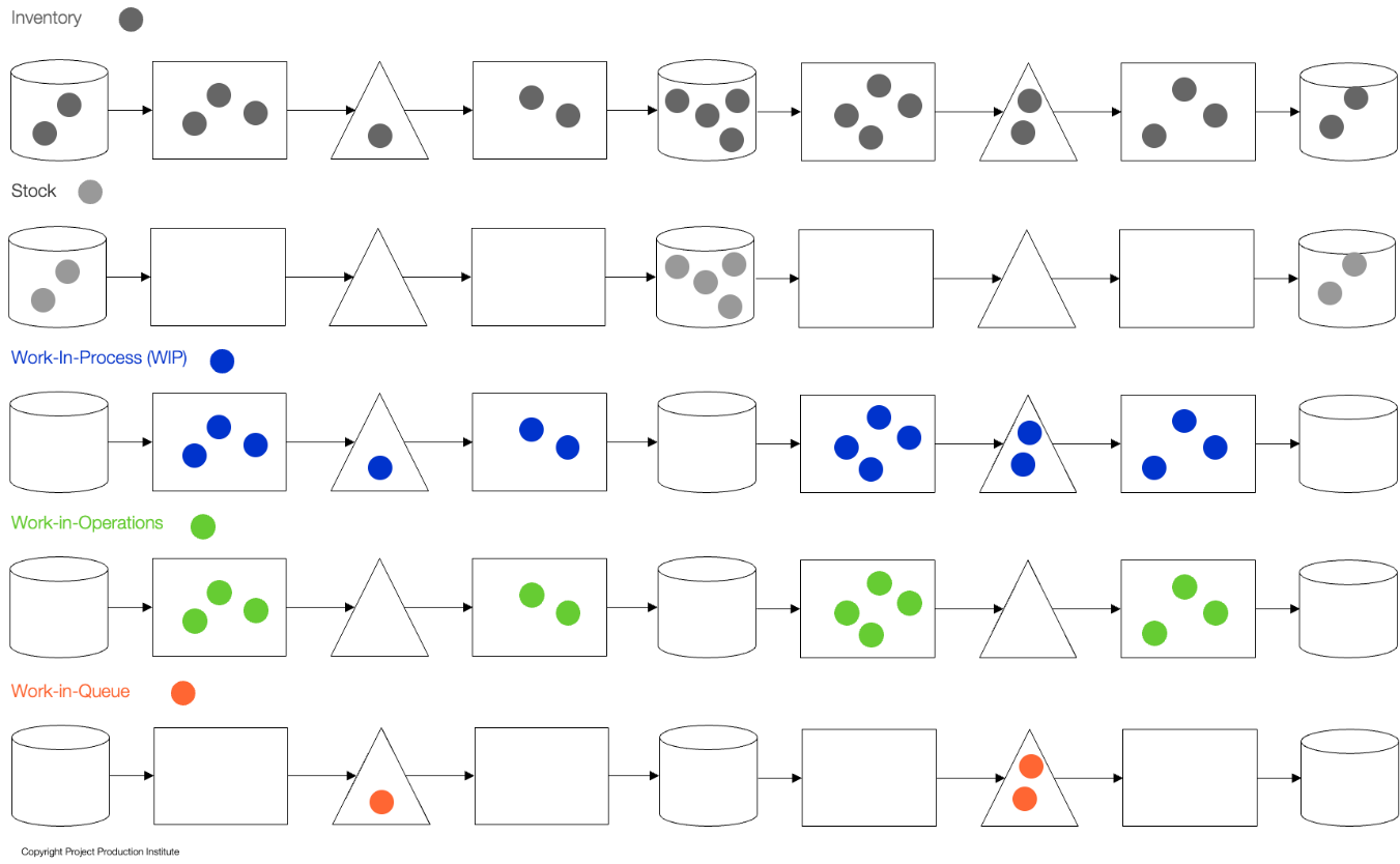
Although these three buffers manifest in individual forms, there is a direct trade-off relationship between inventory (stock) and time. Setting the inventory (stock) policies automatically determines how long the ‘customer’ has to wait. Therefore, Spearman et al. [7] proposed that two buffer decisions have to be made—and not three—namely one pertaining to an inventory-time buffer and the other to a capacity buffer.

The industry’s common use of the term ‘resources,’ which include materials, labor, equipment, time, money, and space, maps to operations science concepts as follows. From a production system perspective, material and information are things that flow through the system in various inventory forms, as raw material or finished products (stocks) or work-in-process. Labor, equipment, and space together determine the capacity of an operation or operations. Money and time are either a constraint to the design of the production system (investment) or an output of the production system design (actual cost and duration of the project).

In project production system design, buffers are design parameters that can be manipulated in different ways. They can be selected by type, inserted at specific locations in the system, sized, and controlled dynamically with policies to meet certain performance objectives, not in the least absorbing variability in the system. For example, dynamic control with real-time feedback using a pull system, possibly enforced with kanban or CONWIP, can limit inventory build-up in the system [8] [9] [10]. As Lean methods for takt planning strive for steadiness and accordingly their objective is to achieve high plan reliability in project delivery, they use capacity buffers, rather than inventory-time buffers to dampen variability [11]. Buffers can be designed-in to govern the interactions between subsystems, for example, “A decoupling buffer is a kind of inventory buffer [stock] in-between two processes, large enough and replenished so that the second process can proceed at its own pace without being held up by the first” [12] [13].

Project production systems in the construction industry have historically-speaking been designed to include inventory- and time buffers, more often so than capacity buffers [14]. However, note that ‘designed’ is not necessarily the correct term here, because inventory and time buffers ‘emerge.’ They can be an unintended consequence of neglect. They will arise when the system is not intentionally designed, i.e., no design decisions are made. That said, when they are designed-in, we speculate that they are favored because they may be perceived as being ‘free’ (from a monetary perspective) whereas the establishment of capacity buffers requires up-front investment and capacity is ‘perishable’ (when it is not used at the time it is available, it is lost). This perception is flawed, however, as it stems from poor accounting practices: e.g., inventory ties up cash (the cost of resources used to produce partially completed products) and occupies space (storage cost) for some amount of time, and the use of space and time also has monetary consequences (opportunity costs, liquidated damages, etc.). In addition, much of the industry’s methodology is geared to maximize labor productivity most of the time through a large inventory buffer to decouple work from upstream variability. However, the result is longer cycle time through the project, not to mention the amount of unproductive capital tied up. In many cases, such intentionally designed solutions may result in unintended consequences.

Alignment of Production System Design with Business Objectives

As mentioned, variability in a production system has to be absorbed by some combination of the three fundamental buffer types. Different combinations are possible, but some will be preferred over others depending on the project context. A tradeoff can be made between buffer types to ensure alignment with the project’s business objective, e.g., time-to-market vs. cost-driven projects. When time-to-market is of the essence (e.g., because of first-to-market opportunity costs), capacity buffers will be preferred over time buffers. This promotes product flow: as soon as a product arrives for processing, the required resource capacity will be available to process it. In contrast, in cost-driven projects where spending is constrained by a limited budget or cost minimization is the objective, time buffers will be preferred over capacity buffers. This promotes high utilization of resources. The purpose of the research is to shed light on such tradeoffs between buffer types.

Parade of Trades

Classic Parade of Trades

To study the preferred use of inventory-time vs. capacity buffers relative to system variability, we created model variants of the Parade of Trades and ran a number of computer-based simulations. The Parade of Trades game has been well described in prior work [5], [4], [15], [16]. It should therefore suffice here to provide a brief overview (adapted from [15]) of the original game formulation nowadays referred to as the ‘Classic Parade.’

The Classic Parade is formed by lining up five trades in a linear sequence (A, B, C, D, and E); these trades perform consecutive steps in a process. The work of each trade is done stepwise (one step per time unit, e.g., one step each week), as is represented by the symbols labeled TradeA through TradeE in Figure 2 (these symbols are called combi activities in the EZStrobe simulation system [17]). The objective is for each trade TradeY to pass 100 units of work from BufferXY in front of them to BufferYZ following them (these symbols are called queues), and thus for the Parade to pass all 100 units from the front of the line (the input buffer, InputA) to the end (the output buffer, TotalE). When this has been accomplished, the project is completed. In this model, all outputs are considered to be made-to-order, and no prepositioned stocks exist between the operations other than the ‘raw material’ in Input A. Therefore, any inventory created will have been backordered and will require time to produce.

Variability is introduced in the simulation by having the roll of a die determine how many work units each trade can pass at a given time. After a trade has rolled her die and passed the appropriate number of units of work, she must wait until the trade downstream from her in turn has rolled her die and taken units of work from the buffer between them, before she may replenish this buffer. During the simulation, participants collect data to analyze and discuss once their project has been completed. Before reading on, readers should familiarize themselves with the original Parade’s details and teaching points presented in [4] and [5].

Using operations science terminology, the Parade’s simple project network as depicted is a 5-trade line-flow with sequential dependence between workstations TradeA and TradeB, etc. Process variability is modeled by sampling randomly from a known binary distribution, e.g., {4, 6} or {3, 7}. InputA and TotalE are stocks. BufferAB, BufferBC, BufferCD, and BufferDE hold inventory (Figure 3).

Note that the Parade of Trades is not a steady-state system, i.e., there is no long-enough sustained period between the ramp-up and ramp-down where average WIP, throughput, and cycle time settle to stable values; therefore, the generalization known as Little’s Law [18] does not directly apply here.

Simulation Data and Performance Metrics

With the intent to study the relationship between inventory-time vs. capacity buffers, the simulation was programmed to track the following data:

1. Time at which each trade mobilizes and demobilizes, from which the ‘trade time on site’ is computed , namely Trade Time on Site = time of trade demobilization – time of trade mobilization.
2. Rolled capacity, passed units, and lost capacity for each trade and each time period.
3. Inventory between trades each time period, so that the integral of the amount of inventory over time is an indicator of the inventory carrying cost.
4. Project duration, namely the time needed to pass all 100 units from the start of the Parade, InputA, to the end, TotalE.

The three metrics reported in this paper, according to which system performance is gauged are:

1. The average amounts of time trades are on site, which is the sum of the average amount of time each trade is on site.
2. The average inventory build-up over time for the project, which is the sum of the average inventory build-up in each of the queues BufferAB, BufferBC, BufferCD, and BufferDE.
3. The average duration to complete the project.

Model Variants of the Classic Parade with Time Buffers

We have been studying variants of the Classic Parade model. Some have included the provision of stand-by capacity (aka. swing- or recourse capacity) as the means to absorb variability while emulating a system that is orchestrated by means of a takt [15], whereas others have included the use of different transfer batch sizes [16]. Here we present variants that have different time buffers, and consequently differ in inventory buffers and thus capacity utilization. Time- and inventory buffers go hand-in-hand as time allows for inventory build-up; we therefore refer to them in combination as inventory-time buffers.

The simulation results for each time-buffer variant are labeled by means of the die used followed by the time at which each of the trades mobilizes, ready to work. For example, the Classic Parade is labeled with the mobilization timing ‘0-1-2-3-4’ to indicate that Trade A mobilizes at time 0, Trade B mobilizes 1 time unit later, Trade C mobilizes 2 time units later, etc. There is no point for Trade B to mobilize to site sooner (which would be at time 0 rather than time 1), because according to the Parade’s network structure they need to wait in any case for the first handoff from A. Likewise, there is no point for Trade C to mobilize at time 0 nor at time 1; the time for C to mobilize is when they can reasonably expect to have received a first handoff from their predecessor, which is at time 2. Similarly, Trade D can reasonably expect to have received a first handoff from their predecessor at time 3, and Trade E at time 4. Using this notation for labeling variants, the Classic Parade with an all-5 die is labeled a ‘5-5 0-1-2-3-4,’ with a 4-6 die as ‘4-6 0-1-2-3-4,’ and so on.

For variants of the Classic Parade, one or several trades are allowed to mobilize one- or several time units later than when they can reasonably expect to have received a first handoff from their predecessor; i.e., they include time buffers. For example, model variant ‘4-6 0-1-2-3-6’ refers to a Parade in which Trade E is time-buffered by 2 units. That is, Trade E will mobilize 2 time units later than the time they could reasonably have expected a first handoff (they would have expected this handoff and therefore would have mobilized at time 4 in the Classic Parade, so now they mobilize at time 4 + 2 = 6). Many model variants with time buffers for one or several trades were simulated, as will be reported in this paper.

Trades stay on site until they have passed 100 units and then immediately demobilize. The time between their mobilization and demobilization is called the Trade’s Time on Site.

In addition to the modeling assumptions presented so far, we made an assumption about the trades’ use of their time. Each trade needs time to take units from their input and transfer them to their output (the duration of any combi TradeY) (possibly called ‘direct work’). They also need time to roll their die (akin to incurring time for planning, setup, and changeover). Given that each cycle takes 1 time unit (e.g., 1 week), it is assumed that the input-to-output time spans 80% of it (0.8 time units) and the time-to-roll 20% (0.2 time units). As per the model this means that inventory between trades (time in the BufferXY queue) will be held for at least 0.2 time units, and longer depending on the follow-on trade’s withdrawal rate.

In the strict sense, one might have expected in the Classic Parade that each trade would take the entire cycle time as input-to-output time and that the time-to-roll might happen ‘in no time’ (like runners in a relay race), with 0 time units for holding inventory. If that were the case, then the Classic Parade with the all-5 die would have only a stock of materials at the start and end, and no inventory in any of the BufferXY queues. This would be highly unlikely in practice and it is not how these durations are modeled here. As modeled, there will be inventory build-up for some amount of time (0.2 time units), even in the Classic Parade with the all-5 die.

Computer Implementation

The discrete event simulation model used to generate data for each of the variants as described was implemented using the EZStrobe Version 4.20 front-end in Microsoft Visio LTSC Standard 2021, and EZStrobe calls the Stroboscope Simulation System Version 5,25,4,1 developed by Julio C. Martinez and Photios G. Ioannou [19]. To allow for matched comparisons, each trade is modeled to have their own die with a dedicated stream of random numbers.

Simulation Results

Table 1 shows the results of numerical simulation of 25 model variants with the all-5, 4-6, and 3-7 dice and using various time buffers. These are average values. Each one of the 4-6 and 3-7 variants was replicated 2,500 times to achieve a tight confidence interval, but to avoid cluttering the table we left standard deviations off.

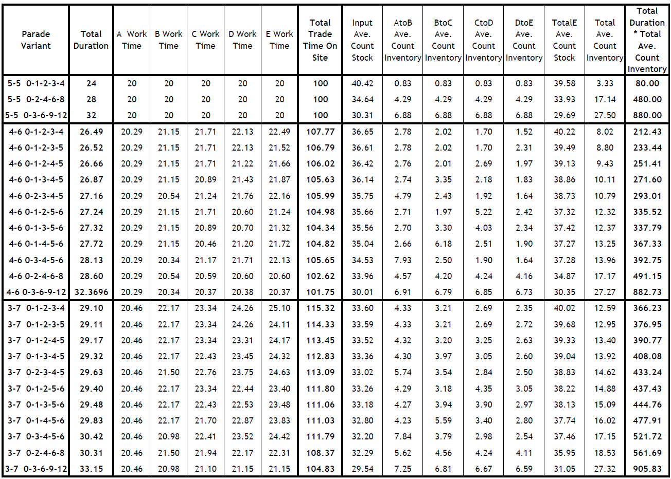
Figure 4 plots data selected from this table. Shown in black (scale at the bottom) is the average Total Duration. Shown in blue (scale at the left) is the sum for all 5 trades of their average Trade Time on Site. Shown in orange (scale at the right) is the average inventory-time that builds up between trades in the four buffers (BufferAB, BufferBC, BufferCD, and BufferDE) during the simulation.

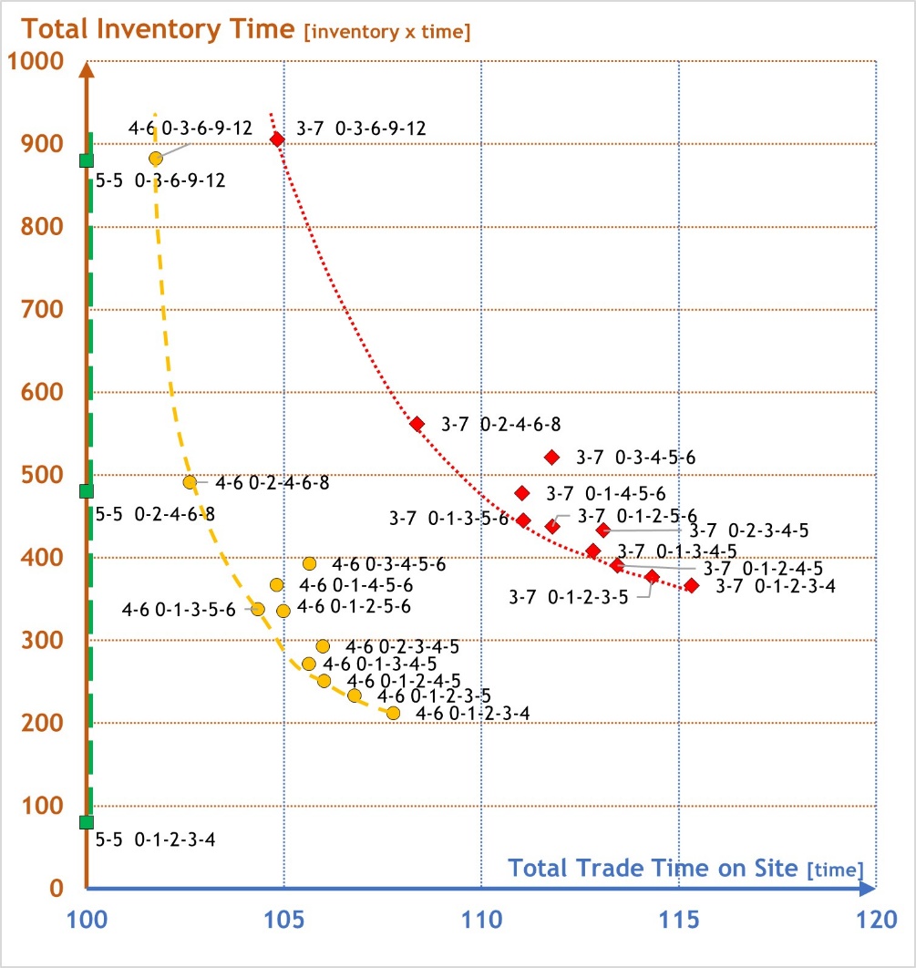
Figure 5 depicts the simulation results in a different way, namely as the Total Trade Time on Site multiplied by the (Total Duration x Total Average Count of Inventory).

The data points obtained using the all-5 die are marked by means of a square, those using the 4-6 die by a circle, and those using the 3-7 die by a diamond. Dashed curves have been added manually to each figure in order to delineate a Pareto optimal front (as will be expanded on later). The differences in curvature, length, and location of these lines on the figures make the impact of variability on system performance clear.

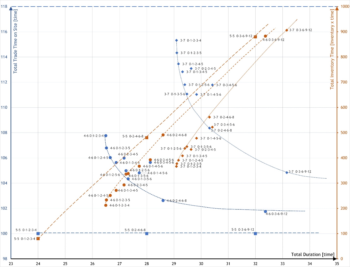
The all-5 variants serve as reference points, indicating the best possible outcomes since no variability is present in the system to hamper performance—a hypothetical case that will never present itself in reality. The data points for the Classic Parade with the 5-5 0-1-2-3-4 model variant can be calculated by hand. As for its project duration, Trade A and every follow-on trade pass 5 units each cycle from their input to their output, so that each one need 20 cycles to complete their work. As four trades follow Trade A, this variant takes 20 + 4 = 24 cycles (24 time units) to complete. With 5 trades in the Parade, the Total Trade Time on Site for all trades combined is 5 x 20 = 100. As for inventory accumulation (work in queue), each cycle, 5 units of inventory will be held for 0.2 units of time in the buffer between subsequent trades. The time-average of the Total Inventory is therefore (20 cycles x 4 buffers x 5 units/cycle x 0.2 time units)/24 time units = 3.33 units. These calculated values are shown on row 1 in Table 1 and by means of the blue square and the orange square in the lower-left of Figure 4. Other variants of the all-5 die are identical in terms of the Total Trade Time on Site, but will take more time in total duration and have more inventory build-up (dashed blue horizontal line in Figure 4 and dashed green vertical line in Figure 5).

Observations And Takeaways

Despite the fact that the Parade of Trades is a very simple, linear system, some of the simulation results may surprise the reader. First, these results show non-linear relationships between the outputs depicted in Figure 4 and Figure 5. This perhaps counter-intuitive observation reflects the combined effect of variability and the structure of the system (sequential dependencies with tighter or looser coupling between trades, depending on the variant).

Second, the mean value and standard deviation of the duration of Trade A for these variants are the same because A is unconstrained. The 100-unit inventory is available to Trade A from the start. In contrast, the duration of all subsequent trades will vary depending on where time buffers have been added (Table 1).

Third, if and when all trades mobilize and start to work as soon as possible, then the project will finish as fast as possible but, due to variability in the system, capacity will inevitably be lost. To illustrate, Figure 4 shows that model variants with mobilization timing 0-1-2-3-4 have the shortest Total Duration and they have the highest Total Trade Time on Site when compared to other variants with the same die.

Similarly, when the start of work gets delayed (following a planned time lag, i.e., buffered with time), the project will take longer to finish but less capacity will be lost; therefore, capacity utilization and thus trade productivity will be greater. This is because the insertion of a time buffer allows inventory to build up so that the trade immediately following the time buffer will be shielded from upstream variability and consequently have a lower likelihood of starving. The degree of shielding will depend on the size of the buffer.

Fourth, less capacity will be lost when the system has less variability for a given time buffer. To illustrate, compare the difference between the baseline of 100 units of Total Trade Time on Site for the variant 5-5 0-1-2-3-4, to 107.77 units needed to deliver 4-6 0-1-2-3-4 (7.77% more) and 115.32 (15.32% more) for 3-7 0-1-2-3-4.

Fifth, even when inserting large time buffers to shield trades from upstream variability by inventory build-up, there will still be lost capacity. Large time buffers also increase the project duration. To illustrate, compare the difference between the three 0-3-6-9-12 variants. They all have a project duration of more than 30 time units. The Total Trade Time on Site is 100 units when using the 5-5 die, 101.75 when using the 4-6 die and 104.83 when using the 3-7 die. They all build up an inventory of more than 27 units.

Sixth, the practice of time buffering is more impactful in reducing Total Trade Time on Site in systems that have more variability. The corollary is that the range of possible capacity loss in case of a delayed start is smaller when the system has less variability. To illustrate, compare the difference in range of the Total Trade Time on Site between 4-6 0-1-2-3-4 and 4-6 0-3-6-9-12 (107.77 – 101.75 = 6.01) with the difference in range between 3-7 0-1-2-3-4 and 3-7 0-3-6-9-12 (115.32 – 104.83 = 10.49).

Seventh, building on the previous two takeaways, it is obvious that increased efforts to optimize for capacity utilization (lowering Total Trade Time on Site) get penalized by increases in time delays and inventory build-up.

Eighth, when adding a time buffer in the Parade, the location of that buffer matters. The simulation results differ depending not only on whether a buffer gets added but also where that buffer is positioned in the system structure. Adding a buffer protects the immediately succeeding trade, as mentioned. Also, because that trade thus is exposed to less upstream variability, they have less variability to pass further down the Parade. This benefit gets attenuated when moving further away from the buffered trade (akin to some kind of bullwhip effect, if that is the term to use here). To illustrate, compare the variants 0-1-2-3-5, 0-1-2-4-5, 0-1-3-4-5, 0-2-3-4-5 for any die and focus for example on Trade E’s work time on site. That work time is smallest when E is the buffered trade, it is slightly larger when D is the buffered trade, slightly larger again when C is, and likewise when B is. Of note is that the ‘best’ position to add a time buffer to a Parade will vary based on the length of the Parade because two effects are at play: (1) the benefit of buffering a trade and (2) the number of trades downstream that also benefit from this buffer.

Ninth, if we look at capacity expressed in die rolls, each Parade variant can be considered balanced in the sense that the dies used by the trades all have the same mean and standard deviation, regardless of which die is used {5}, {4, 6}, or {3, 7}. The results show that in the face of variability, a balanced production system may not be the best production system design since the trade outputs are very sensitive to variability.

Last but not least, we manually added dashed curves to each figure to delineate a Pareto optimal front. Each die (coefficient of variation 0 for the all-5 die, 0.2 for the 4-6 die, and 0.4 for the 3-7 die) has its own front. For a given level of variability in the system, this front defines the possible tradeoff choices between Total Trade Time on Site and Total Inventory Time. The front would move if variability in the system were to change. To illustrate, variants 0-1-2-3-4, 0-1-2-3-5, and 0-1-2-4-5 define the front; however, variants such as 0-2-3-4-5 and 0-3-4-5-6 are clearly inferior. Consequently, when designing a project production system and recognizing the expected amount of variability, managers must choose where they wish to operate on their Pareto front to meet their business objectives and accordingly structure their system with the appropriate buffers.

Applications In Practice

The aforementioned observations and takeaways have focused on capacity utilization (Trade Time on Site) and project duration, yet also referred to inventory build-up. From an operations science perspective, inventory (stock) sizing and positioning is a key concern in production system design. This notwithstanding, in capital project management it is still uncommon to place much if any attention on inventory: construction project planning and scheduling tools tend not to model or depict inventory build-up at all. More often than not, having inventory on site is considered progress (as it should), and most often it increases value earned. However, not much consideration is given to how much is the right amount until there is shortage of laydown or staging area. This is a major oversight because inventory defines handoffs and affects whether and when succeeding trades can work. In addition, the physical and virtual build-up and management of inventory require resources and comes at a cost (space use, handling effort and transportation distance, cost of goods awaiting further processing, etc.). As Figure 4 and Figure 5 illustrate, capacity utilization and inventory have an inverse relationship: one will offset the other; both must be taken into account when optimizing the system to meet certain performance objectives.

This issue is exacerbated when the items to be engineered, produced, delivered, and installed are unique (e.g., pipe spools, modules, and permanent equipment) and must be placed in a certain sequence in a designated location. Just managing the total quantity does very little for the installation process. If it is important to the project to minimize inventory and associated costs, tied-up cash, as well as the potential risk of obsolescence from design changes, through synchronizing engineering, fabrication, delivery, and installation, then having right-sized capacity buffers at the right locations will likely outperform inventory buffers in minimizing value stream cost.

Consider for example the rebar production system design and control deployed at Heathrow Terminal 5. Details regarding the strategies, approaches, and policies for the design and control of the production systems for this project are beyond the scope of this paper, but pertinent information regarding the rebar production system is described next. Key considerations and constraints that shaped the design of the rebar production system included:

Demand Forecast

• Cut, bent & loose rebar: 200 tons per day
• Pre-assembled rebar cages: 113 tons per day

Delivery Constraints

• Surrounded by Europe’s busiest motorways
• Single point of ingress/egress
• Expected rate of deliveries during civil phase: One every 30 seconds
• Deliveries not allowed between 7:00 AM – 9:00 AM and 4:00 PM – 6:00 PM
• Heightened security

Site Constraints

• 80 subprojects simultaneously executed on site
• Site storage limited to one day’s worth of work

With the goal of getting “the right information, the right materials, the right labor and the right equipment, in the right quantity delivered to the right place at the right time, every time,” the chosen approach for mitigating detrimental variability while absorbing remaining variability was to use capacity buffers and raw material buffers. Although many physical and digital assets had to be properly designed and configured to make this possible, the execution process is worth highlighting here.

The Project Production Control solution ensured the site execution team could send highly reliable demand information on which rebar elements and assemblies would be needed one week out. Rather than engineering, fabrication, and logistics teams having their own schedules, they were configured with appropriate capacity buffers to respond to demand without batching or resequencing, optimizing their individual productivity. This was supported by having an appropriate amount of raw material delivered through a rail system backed up by trucks for redundancy.

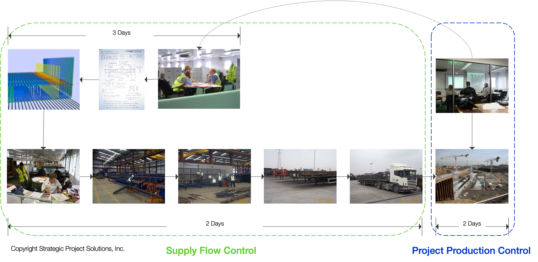
This production system contributed to BAA opening Heathrow’s fifth terminal for business on 27 March, 2008, after six years of construction at a cost of £4.3 bn, on time and within budget. As for the cost of the rebar production system, the project reported it was the most expensive per ton of rebar fabricated but the cheapest per ton of rebar fabricated, delivered and installed, a.k.a., value stream cost.

As for other construction project planning practices such as Advanced Work Packaging (AWP), as defined by the Construction Industry Institute (CII) and the Construction Owners Association of Alberta (COAA) [20] [21], they are advocating for the protective use of time buffers in schedules in an effort to maximize on-site tool time. Some AWP practitioners have set time-based policies such as maintaining a 3-to-4-week backlog of fully developed, constraint-free Installation Work Packages (IWPs), yet they do not provide a mathematical rationale from a production perspective. Notably, the guidance for AWP provided in the 3 volumes of more than 400 pages in total [20] and the summary of 28 pages [21] mentions the word ‘complexity’ only 7 times, ‘uncertainty’ 1 time, ‘variability’ 1 time (“variability in AWP practice”), ‘inventory’ 2 times, and ‘risk’ 25 times. Without the conceptualization and explicit acknowledgment of the occurrence of variability (and related concepts), and given the impact variability is known to have on production system performance [2]—as illustrated in this paper with a very simple model—clearly the AWP guidance does not size its buffers to the variability they are meant to absorb [22] [23].

Having realized this gap, the AWP community has been taking steps to integrate AWP, Lean Construction, and Project Production Management for the benefit of the industry. Lean thinking in construction (e.g., the Last Planner System with pull planning and the use takt planning with capacity buffers) and operations science are reshaping current thinking about AWP [24] [25] [26] [27] to define AWP+. They add control mechanisms and a theoretical mathematical basis to size inventory, time, and capacity buffers to enable a smooth workflow without bloating site inventory.

Conclusions

The Parade of Trades is intentionally a simple system, including a line-up of only five trades and a simple source of variability, namely randomness introduced by rolling a die (or flipping a coin). Thanks to its simplicity, the simulation helps develop intuition about the impact of managerial actions on project production systems’ performance. The Parade emulates a project-based production system with a relatively short time frame so that no steady state is reached. Even for a simple, linear system as exemplified by the Parade, the presence of variability results in non-linear system behavior.

The objective of the computer-based simulations of 25 variants of the Classic Parade of Trades model was to obtain data that illustrates the detrimental impact variability has on a system’s performance. The tight interdependence with finish-to-start relationships between sequential trades in the production system was relaxed by adding time buffers. Depending on the coefficient of variation that characterizes the system and on business objectives, one means of buffering may be preferred over another. More loose coupling of interdependencies allows for greater capacity utilization but is at odds with any pressure to deliver projects fast. The two figures illustrating Pareto optimal fronts confirmed a lesson from Factory Physics [2]: You will pay for variability one way or another.

Project managers can use the findings from this simulation to select management approaches better-suited for their project-specific context and chosen performance objectives, while recognizing that variability will degrade their project production system’s performance.

Acknowledgments

This study on the use of inventory-time buffers vs. capacity buffers in production systems subject to variability was supported by contributions from the Project Production Institute (PPI) and other members of the Project Production Systems Laboratory (P2SL) at the University of California, Berkeley. We express our sincere thanks for all the support we received. Any opinions, findings, conclusions, or recommendations expressed in this paper are those of the authors and do not necessarily reflect the views of contributors to P2SL.

Data Availability

To request copies of the model variants programmed in EZStrobe [17] please reach out to the first author.

References

1. [1]G. Ballard and I. D. Tommelein, “2020 Current Process Benchmark for the Last Planner System of Project Planning and Control,” Project Production Systems Laboratory, Berkeley, CA, 2021, https://escholarship.org/uc/item/5t90q8q9.
2. [2]W. J. Hopp and M. L. Spearman, Factory Physics, Third ed., Waveland Press, 2011.
3. [3]D. Chhajed and T. J. Lowe, Eds., “Building Intuition: Insights from Basic Operations Management Models and Principles,” Springer Science & Business Media, 2008, p. 177.
4. [4]I. D. Tommelein, D. R. Riley and G. A. Howell, “Parade Game: Impact of Work Flow Variability on Succeeding Trade Performance,” in Proc. 6th Ann. Conf. Int. Group for Lean Constr. (IGLC6), Guaruja, Brazil, 1998.
5. [5]I. D. Tommelein, D. R. Riley and G. A. Howell, “Parade game: Impact of Work Flow Variability on Succeeding Trade Performance,” Journal of Construction Engineering and Management, vol. 125, no. 5, pp. 304-310, 1999.
6. [6]H. J. Choo, “Beyond Variability - Designing and Controlling Capital Project Production Systems,” in Project Production Institute, Technical Conference, 2026.
7. [7]M. Spearman, M., J. Bell and E. Pound, “Operations Science Applied,” Hercher Publishing Inc., 2026.
8. [8]W. J. Hopp and M. L. Spearman, “To Pull or Not to Pull: What Is the Question?,” Manufacturing & Service Operations Management, vol. 6, no. 2, pp. 133-148, 2004.
9. [9]I. D. Tommelein, “Pull-driven Scheduling for Pipe-Spool Installation: Simulation of Lean Construction Technique,” Journal of Construction Engineering and Management, vol. 124, no. 4, pp. 279-288, 1998.
10. [10]R. Arbulu, “Application of Pull and ConWIP in Construction Production Systems,” in Proc. 14th Ann. Conf. Int. Group Lean Constr. (IGLC14), Santiago, Chile, 2006.
11. [11]A. G. Frandson, O. Seppänen and I. D. Tommelein, “Comparison Between Location Based Management and Takt Time Planning,” in Proc. 23rd Ann. Conf. Int. Group Lean Constr. (IGLC23), Perth, Australia, 2015.
12. [12]Project Production Systems Laboratory (P2SL), “P2SL Glossary,” Project Production Systems Laboratory, [Online]. Available: https://p2sl.berkeley.edu/glossary/knowledge-center-glossaryatoz/. [Accessed 30 05 2026].
13. [13]G. A. Howell, G. Ballard and A. Laufer, “Interaction between Subcycles: One key to Improved Methods,” Journal of Construction Engineering and Management, vol. 119, no. 4, pp. 714-728, 1993.
14. [14]R. Arbulu, “The Batching Frenzy,” in Project Production Institute, 2021.
15. [15]I. D. Tommelein, “Takting the Parade of Trades: Use of Capacity Buffers to Gain Work Flow Reliability,” in Proc. 28th Ann. Conf. Int. Group Lean Constr. (IGLC28), Berkeley, California, USA, 2020.
16. [16]G. F. Saragih and I. D. Tommelein, “Parade of Trades with Transfer Batching,” in Proc. 34th Ann. Conf. Int. Group Lean Constr. (IGLC34), Singapore, 2026.
17. [17]J. C. Martinez, “EZStrobe: General Purpose Simulation System based on Activity Cycle Diagrams,” in Proc. 2001 Winter Sim. Conf., 2001.
18. [18]J. D. C. Little and S. C. Graves, “Chapter 5: Little's Law,” in Building Intuition: Insights from Basic Operations Management Models and Principles, D. Chhajed and T. J. Lowe, Eds., Springer, 2008, pp. 81-100.
19. [19]J. C. Martinez, STROBOSCOPE State and Resource Based Simulation of Construction Processes, University of Michigan, Ann Arbor, Michigan: PhD Dissertation, Civil and Environmental Engineering Department, 1996.
20. [20]CII, “Advanced Work Packaging: Design through workface execution. Implementation Resource 272-2, Version 3.0, Volumes I, II, III,” Construction Owners Association of Alberta (COAA) and Construction Industry Institute (CII), Austin, Texas, July 2013.
21. [21]CII, “Advanced Work Packaging: Design through workface execution. Research Summary 272-1. Version 2.0,” Construction Owners Association of Alberta (COAA) and Construction Industry Institute (CII), Austin, Texas, July 2013.
22. [22]G. Ballard and I. D. Tommelein, “A Critique of Advanced Work Packaging,” Project Production Institute, 2015, https://projectproduction.org/wp-content/uploads/2017/11/A-Critique-of-Advanced-Work-Packaging.pdf.
23. [23]I. D. Tommelein and G. Ballard, ““Advancing” Advanced Work Packaging (AWP),” Journal of Project Production Management, vol. 1, 2016.
24. [24]CII, “AWP + Lean: Exploring Opportunities - Better Together. Special Report 22-01a,” Construction Industry Institute and Lean Construction Institute, Austin, TX, 1 December 2022.
25. [25]CII, “AWP + Lean: Exploring Opportunities - Organizational Culture. Special Report 22-01b,” Construction Industry Institute and Lean Construction Institute, Austin, Texas, 1 December 2022.
26. [26]D. Fauchier and L. Rankin, “Work Packaging (AWP) and Lean Construction: A Comparison of Approaches. SR 22-01c,” Construction Industry Institute and Lean Construction Institute, Austin, Texas, 10 February 2023.
27. [27]F. Espana and J. Strickland, “Advanced Work Packaging (AWP) and Lean Construction: Optimizing Project Workflow,” Construction Industry Institute and Lean Construction Institute, Austin, Texas, 23 August 2023.