
Rates and ratios are used extensively throughout the engineering and construction industry, but the terms are often associated with commercial, financial, or administrative measures such as labor rates, equipment rates, billing rates, overhead rates, cost expenditure rates, productivity factors, time on tools ratio, and other project management measurements. While these measures are important, they do not explain how work flows through the production systems that ultimately deliver project outcomes.
Production measurements, by contrast, are fundamental properties of production systems regardless of industry or application. From an Operations Science and Project Production Management (PPM) perspective, projects can be understood as networks of interconnected production systems configured to deliver a specific outcome. Some of these systems are non-physical, such as engineering and design processes that transform requirements into deliverables. Others are physical, such as fabrication, assembly, installation, and commissioning processes that transform materials, components, and systems into operational assets. Regardless of their nature, production system behavior is determined not only by the rates at which work is required, processed, completed, reworked, or rejected, but also by operating parameters such as Work-in-Process and Capacity Utilization. Work-in-Process can be directly influenced through work release and production control policies, while Capacity Utilization can be intentionally designed by balancing the Load imposed on the system with its available Capacity. Together, these parameters shape Throughput, Cycle Time, queue formation, responsiveness to variability, and overall delivery reliability.
This paper proposes six fundamental measurements that characterize how work flows through the production systems: Demand, Capacity, Throughput, Load, Rework, and Scrap. Although these measurements are applicable to production systems more broadly, the discussion is framed in the context of engineering and construction projects. The paper presents a technical framework for understanding, differentiating, and applying these measurements together with Work-in-Process and Capacity Utilization when designing, configuring, controlling, and improving production systems. By distinguishing production rates, ratios and operating parameters from administrative and financial measures, it provides engineering and construction professionals with a more direct means of diagnosing bottlenecks, selecting appropriate operating conditions, anticipating performance issues, and improving the predictability and reliability of project delivery.
Keywords: Capacity, Demand, Load, Measurements, Production Systems, Rates, Ratios, Rework, Throughput, Scrap.

Roberto Arbulu is Senior Vice President of Technical Services for Strategic Project Solutions. He has more than twenty years of experience in the delivery and optimization of energy, industrial, technology, and infrastructure capital projects and has worked with numerous owner operators and service providers across North America, South America, Europ ...
The engineering and construction industry makes extensive use of measurements or key performance indicators. Most practitioners are familiar with measurements including rates and ratios associated with project administration and management, such as labor rates, equipment rates, billing rates, overhead rates, cost expenditure rates, productivity factor, time on tools ratio, and various project performance metrics. These measures are essential for estimating, budgeting, reporting, and project controls because they quantify the financial, commercial, and administrative aspects of project delivery. However, while they describe how projects are planned, funded, and managed, they provide only limited insight into how work actually flows through the production systems [2] responsible for delivering project outcomes.
This paper does not address the use of these administrative and financial rates. Instead, it focuses on project production systems and examines the role fundamental measurements play in transforming inputs into outputs to achieve a desired outcome. Production measurements are inherent properties of production systems and are fundamental to understanding production performance. They describe the rate at which work is required, the rate at which a production system is capable of producing, the rate at which it actually produces, the rate at which work is imposed on its operations, and the losses associated with rework and scrap. Collectively, and together with other production measurements such as Capacity Utilization (CU) and Work-in-Process (WIP), these measurements explain how work flows through production systems and why projects succeed or fail in achieving planned outcomes.
This distinction has important practical implications. Administrative measures remain essential for managing the commercial and financial aspects of projects, while production measurements provide the technical basis for designing, validating, controlling, and improving the production systems that ultimately determine project performance. Consequently, production measurements should not replace traditional estimating and scheduling practices; rather, they should complement them by ensuring that project budgets and schedules are grounded in the demonstrated capability of the production systems expected to deliver the work.
Schedule delays, cost overruns, and productivity losses rarely occur randomly [1]. They typically emerge from mismatches between the output required by a project and the output that its production systems can deliver. Production measurements provide a direct means of understanding, diagnosing, and managing those mismatches. Unlike many project management metrics, which often serve as lagging indicators of performance, production measurements provide direct insight into the behavior of production systems and their ability to satisfy project objectives.
While rates alone do not determine production system performance – CU, WIP, variability, among other factors, also play a critical role as it will be further described later in this paper – they provide a foundational framework for understanding the relationship between desired and actual system behavior. This paper introduces and differentiates six fundamental measurements commonly found in production systems and seeks to develop intuition and practical understanding of how to evaluate, design, control, and improve them through the lens of these measurements.
Most of the outcomes that Project Managers care about - schedule performance, cost performance, workflow reliability, and predictability - are emergent properties of the production systems operating within the project. Production measurements provide visibility into those systems long before schedule or cost reports reveal a problem.
Production measurements determine what a production system must deliver, what it can deliver, and what it is actually delivering. They reveal whether project commitments are achievable, where bottlenecks exist, and how losses such as rework and scrap affect performance. While cost and schedule metrics primarily reflect the consequences of production system performance, production measurements provide insight into the mechanisms that drive that performance. Consequently, production measurements can reveal future production constraints long before they manifest as schedule delays or cost overruns.
Viewed through this lens, production measurements explain how work flows through project production systems and why projects succeed or fail [1] in achieving planned outcomes. Understanding and managing these measurements enables project teams to identify constraints, anticipate performance issues, and improve the predictability and reliability of project delivery.
Engineering and construction projects are managed through two complementary but fundamentally different systems: a management system, responsible for planning, coordinating, administering, and monitoring project execution, and a production system, responsible for designing, engineering, fabricating, assembling, installing, commissioning, and ultimately delivering the asset. Each requires its own set of measurements because each serves a different purpose.
Project Management measures provide visibility into the planning, scheduling, administration, coordination, and commercial performance of a project. They include financial measures, cost and schedule performance metrics, staffing levels, procurement status, document processing metrics, and planning and execution measures such as labor billing rates ($/hour), equipment rates ($/hour), expenditure rates ($/day), earned value indices (CPI and SPI), RFI closure rates (RFIs/week), procurement processing rates (purchase orders/week), Time on Tools (workforce effectiveness metric measured typically as percentage), Productivity Factors (earned vs. burned), and Takt (planning and synchronization parameter measured as time / unit or unit / time depending on convention, but not a physical property of the production system itself). Collectively, these measures support estimating, planning, reporting, governance, forecasting, and commercial management.
Although several of these measures are mathematically expressed as rates or ratios, they should not be confused with the production rates that govern the behavior of production systems. Project Management measures primarily describe how a project is planned, managed, administered, financed, synchronized, or monitored. Production rates, in contrast, describe the movement and transformation of work through the interconnected production systems that create project value.
This distinction is very important because project outcomes ultimately emerge from the performance of production systems rather than from the management systems used to observe them. Cost reports, earned value metrics, staffing reports, productivity indicators, time on tools, and takt compliance provide valuable insight into project execution; however, they generally reflect planning assumptions, management performance, or the consequences of production system behavior. On the other hand, production rates, together with WIP and CU, provide direct insight into the capability of production systems to satisfy Demand, utilize Capacity, sustain Throughput, absorb variability, and achieve the production objectives established by the project.
The objective of this paper is therefore not to diminish the importance of project management measures. Rather, it is to emphasize that they complement a distinct class of measurements grounded in Operations Science that govern the behavior of production such as engineering, fabrication, assembly, testing, transport, installation, commissioning. Understanding and managing these production measurements provides a more direct basis for explaining, predicting, designing, and improving production system performance, while enabling project management measures to more accurately reflect the underlying realities of project execution.
To summarize, project management measures answer questions about how well the project is being planned, managed, and controlled (as in project controls). Production measurements answer questions about how work flows through the production systems that deliver the project. Both perspectives are necessary, but together with other production measurements (e.g., CU and WIP), production rates provide the fundamental basis for understanding and managing the behavior of the production systems from which project performance ultimately emerges.
Numerous publications by the Project Production Institute (PPI) [2], [3], [4], [5], [6] have established the foundational concepts of Project Production Management (PPM) as the application of Operations Science to projects including methods for representing and analyzing project production systems, and the principles governing production system design, control, and improvement. Rather than revisiting those concepts, this paper builds on that body of knowledge by focusing specifically on the production rates and related measurements used to characterize production system behavior. This section therefore establishes the terminology, units of measure, and fundamental relationships required for the discussion that follows. Readers seeking additional technical background are encouraged to consult the broader body of PPI publications [6].
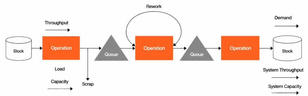
Figure 1 presents the production system representation used throughout this paper. It comprises operations, stocks, queues, and flows - the fundamental elements required to describe how work moves through a production system. From a production perspective, inventory may be physical, such as materials or partially completed assemblies, or non-physical, such as information, design packages, approvals, or test records. Operations transform this inventory into progressively higher-value outputs using resources such as craft labor, knowledge workers, equipment, tooling, and space. As inventory moves through the system, it encounters processing operations, variability, and queues that form and fluctuate over time. The interaction among these elements determines system-level outcomes including Throughput, Cycle Time, Work-in-Process, queue formation, and delivery reliability.

Little’s Law establishes a fundamental steady-state relationship among the average Work-in-Process (WIP) within a production system, the average Throughput (TH), and the average Cycle Time (CT). Provided that the system is observed over a sufficiently representative period and that the same system boundary and unit of flow are used for all three measures, the relationship is:
WIP=TH×CT
This relationship demonstrates that WIP, TH, and CT cannot be considered independently. For a given TH, increasing WIP increases average CT; conversely, reducing WIP without regard to system conditions may starve downstream operations and reduce TH. Little’s Law is an identity, not a control rule. It describes the average relationship among the three variables but does not, by itself, prescribe the amount of WIP that should be maintained.
CU expresses the degree to which available production capacity is committed. At the production-system level, where the project schedule establishes the required output (the Demand), CU may be expressed as the ratio of Demand to system Capacity:
CU = (Demand / Capacity) x 100%
At the operation level, CU is more directly expressed as the ratio of the Load imposed on the operation to its available Capacity, so it can be expressed as:
CU = (Load / Capacity) x 100%
These mathematical relationships should be interpreted carefully. Demand is an external requirement imposed on the production system, not a characteristic of the system. Load is the work released to or required from a specific operation. Capacity is the maximum sustainable output rate under defined operating conditions. CU is therefore a derived, dimensionless ratio rather than a production rate. It cannot be changed directly so project teams influence it by controlling the Load released into the system, changing available Capacity, or both.
WIP and CU have particular importance in production system design and control. WIP can be directly regulated through release policies, pull mechanisms, CONWIP (Constant Work-in-Process) limits, buffer policies, and other production control rules. CU can be intentionally designed by selecting sufficient Capacity and controlling Load so that the system retains protective capacity to absorb variability. Throughput and Cycle Time, by contrast, are emergent performance outcomes produced by the interaction among Demand, Load, Capacity, WIP, variability, reliability, and operating policies. Project teams therefore do not set Throughput or Cycle Time directly; they influence them by changing the controllable conditions under which the production system operates.
| MEASUREMENT | TYPE | UNIT OF MEASURE | EXAMPLE |
|---|---|---|---|
| Throughput | Rate | Units per Time | 20 Modules / Day |
| Cycle Time | Time | Hours or Days | 05 Days |
| Work-in-Process | Quantity / Stocks | Units | 100 Modules |
| Capacity Utilization | Ratio | Dimensionless or Percent | 80% |
Table 1. Representatives Production System Measurements
Accordingly, production rates describe the speed at which work is required, processed, or completed, while WIP and CU help define the operating condition of the production system. Together, these measurements provide a basis for understanding whether a production system can satisfy Demand reliably and how changes in production system design or control are likely to affect performance.
For analytical clarity, the measurements used in production systems should be classified according to their dimensional form. Flow rates express quantities per unit of time, such as modules per day, engineering deliverables per week, or systems commissioned per month. Ratios compare quantities having compatible dimensions and are therefore dimensionless, although they are often reported as percentages; examples include Capacity Utilization, yield, and first-pass quality. Stocks measure the quantity of work or material present within a defined system boundary at a point in time, including WIP, raw material, buffer inventory, and finished goods. Time measures express duration, including Cycle Time, processing time, queue time, setup time, transportation time, and delay.
This dimensional distinction is important because measurements with different units describe different aspects of production system behavior and should not be treated interchangeably. Rates describe the speed of flow, stocks describe the quantity present, ratios describe relative relationships, and time measures describe duration. While every rate is a ratio, not every ratio is a rate. Therefore, maintaining this distinction improves the precision of production system analysis and reduces ambiguity when interpreting performance data.
Independently of the complexity and criticality of a production system, its behavior is influenced by six fundamental production rates: 1) Demand - the output the production system is required to deliver, 2) Capacity - the output the production system is capable of delivering, 3) Throughput - the output the production system actually delivers, 4) Load - the amount of work imposed on resources, including work generated by rework, 5) Rework - the portion of output that re-enters the production system for correction because requirements were not met, and 6) Scrap - the portion of output that is permanently rejected for failing to meet requirements. While WIP and Capacity Utilization complement define the operating conditions under which the production system performs, production rates describe the flow of work through production systems. Additionally, there are other factors that influence production system behavior such as equipment reliability (e.g., failure rates), material replenishment (e.g., fill rates), resource availability, operating policies, and variability (arrival and process). Together, they provide a practical framework for analyzing, designing, and controlling production systems using Operations Science principles.
The fundamental idea is that project schedules establish what must be delivered and when, but production system design, including production rates, determine whether those commitments are physically achievable. Demand rates define the output required from production systems, capacity rates define the output that can be achieved, throughput rates quantify actual performance, and rework and scrap rates reveal losses that consume valuable capacity. While demand, capacity, throughput, and load are measured in units over time, rework and scrap are normally quantified as percentages of the rate of output at a given operation. Although engineering, procurement, fabrication, construction, and commissioning often operate with different metrics, the proposed production rates create a common language as they apply across all phases, disciplines and types of work.
The following table and schematic summarize definitions and units of measure as well as illustrate these six rates using the initial project production system representation.
| RATE | DEFINITION | UNIT OF MEASURE |
|---|---|---|
| Demand | The output the production system is required to deliver | Units / time |
| Capacity | The output the production system is capable of delivering (represents the upper limit of throughput) | Units / time |
| Throughput | The output the production system actually delivers (equals demand or capacity, whichever is less) | Units / time |
| Load | The amount of work imposed on resources, including work generated by rework | Units / time |
| Rework | The portion of output that re-enters the production system for correction because requirements were not met | Percentage |
| Scrap | The portion of output that is permanently rejected for failing to meet requirements | Percentage |
Table 2. Types of Rates, Definitions & Units of Measure
Production systems exist to satisfy demand, regardless of whether they produce directly to customer orders or replenish inventory. Because projects can be understood as temporary production systems, the production systems that comprise a project likewise exist to respond to demand. In project environments, this demand is typically established by the project schedule. Demand establishes the level of output a production system must consistently achieve to satisfy project objectives and maintain schedule commitments.
From an Operations Science perspective, Demand is a fundamental production system parameter because it defines the throughput required for the system to achieve its intended objectives. However, Demand is an external requirement imposed on the production system, not a characteristic of the system. Demand is therefore expressed as a rate - measured as units of output over time. Examples include engineering deliverables required per week, pipe spools fabricated per day, systems commissioned per week, or rooms turned over per month.
Understanding Demand is essential when designing, configuring, controlling, and improving production systems. However, many engineering and construction professionals do not traditionally view projects through a production-system lens. As a result, the concept of Demand is often misunderstood, underestimated, or overlooked altogether.
When actual Throughput consistently falls below Demand, schedule delays become increasingly likely. Conversely, when Throughput meets or exceeds Demand, the production system can support the planned rate of project delivery. In some cases, excess Throughput capability may also reveal opportunities to reduce costs by eliminating unnecessary capacity or release work earlier (if the subsequent production processes have the Capacity to take and process the extra work output that they may receive).
Because Demand is expressed as a rate, it is calculated by determining the quantity of output required over a specified period. Project schedules typically define the timeframe within which work must be completed and may also identify the associated quantities. However, schedules often specify only scope and required completion dates. In such cases, quantities must be obtained from supporting sources such as Bills of Quantities (BOQs), Bills of Materials (BOMs), design deliverable registers, procurement plans or registers, or commissioning plans, fishbones or similar.
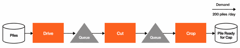
Consider a simple example. Assume a project schedule requires the installation of 10,000 precast piles over a ten-week period. The resulting average Demand is 1,000 piles per week. Assuming a five-day workweek and an even distribution of Demand, the Demand rate becomes an average of 200 piles per day. In production system terms, the system must be designed, resourced, and controlled such that an average of 200 completed piles leave the system every working day.
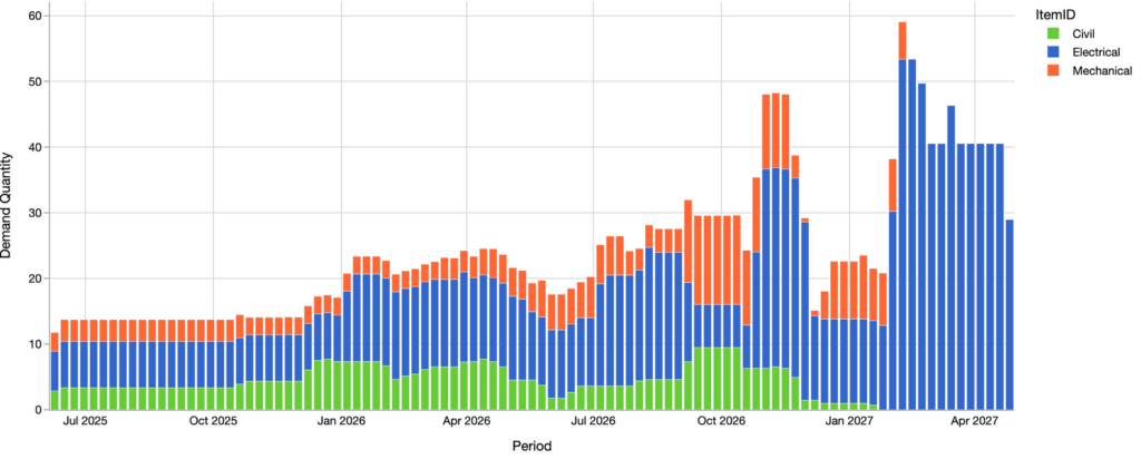
In practice, however, Demand is rarely distributed evenly over time. The Demand imposed by project schedules is often highly variable, with periods of low Demand followed by significant peaks. Production systems must therefore be capable of responding to changing Demand levels while maintaining acceptable performance. Furthermore, variability in Demand introduces additional challenges, as it can significantly impact flow, capacity utilization, inventory levels, and cycle times. To illustrate this point, consider the Demand profiles shown in the examples below, derived from actual projects. The first example depicts the Demand imposed by a schedule on an engineering production system. Demand quantities for three categories of engineering deliverables are plotted over time. The profile reveals that Demand increases substantially toward the end of the planned production period, reaching levels two to three times higher than those required at the beginning of the engineering phase. Such Demand patterns have important implications for aspects like production system design and capacity planning, and they highlight the importance of understanding Demand as a dynamic rather than static parameter.
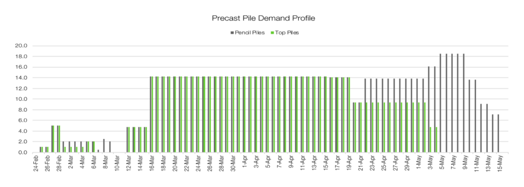
The second example shown in Figure 5 depicts the Demand imposed by a project schedule on a piling production system. In this case, the schedule establishes varying Demand levels for two different pile types to be installed over an approximately three-month period. Consequently, the production system must be capable of delivering the required quantities of each pile type while responding to the fluctuations in demand reflected in the profile.
This piling production system extends beyond on-site installation activities and includes all processes required to transform raw materials into completed installations, including fabrication, assembly, transportation to site, and final pile installation. As such, the Demand profile affects not only field operations but also upstream production activities throughout the entire production system. An additional challenge arises because certain resources may be shared between the two pile types. For example, fabrication facilities, transportation assets, installation crews, and specialized equipment may be required to support both Demand streams simultaneously. As Demand fluctuates over time, competition for these shared resources can create capacity constraints, bottlenecks, and disruptions if not properly anticipated and managed.
Understanding the Demand profile is therefore essential for production system design and control. It enables project teams to assess whether available Capacity is sufficient, determine when additional resources may be required, identify potential bottlenecks, and develop strategies to maintain flow and meet schedule commitments despite variations in Demand. Demand is also a critical production system parameter because it directly influences the amount of work-in-process (WIP) required for the system to operate effectively. According to Little’s Law, Throughput, Cycle Time, and WIP are fundamentally related. Consequently, the level of Demand placed on a production system helps determine the optimal amount of WIP necessary to sustain the required Throughput and achieve planned production objectives.
Maintaining an appropriate level of WIP is critical because both insufficient and excessive WIP can degrade system performance. When WIP is too low, downstream operations may become starved of work, reducing Throughput and causing resources to remain idle (low-capacity utilization levels). Conversely, excessive WIP increases cycle times, creates congestion, and ties up capital in partially completed work. In project environments, excessive WIP can also reduce visibility, complicate coordination, and increase the likelihood of rework and schedule disruption.
Determining the optimal WIP level therefore requires balancing Demand, Capacity, Throughput, and variability within the production system. Because Demand establishes the Throughput required from the system, it serves as a fundamental input when designing and controlling WIP levels. Readers interested in the underlying methodology are encouraged to consult PPI publications that address production system design and optimal WIP determination in greater detail.
Throughput represents the actual output rate achieved by the system. More specifically, Throughput is the average rate at which conforming units are completed by the production process, excluding defects, rework, and other outputs that fail to meet requirements. Throughput is therefore a measure of current system performance. It quantifies how many good units are produced over a given period, such as an hour, a day, or a week. For example, if a piling production system completes 750 piles that meet project specifications over a five-day workweek, its average Throughput is 150 good piles per day.
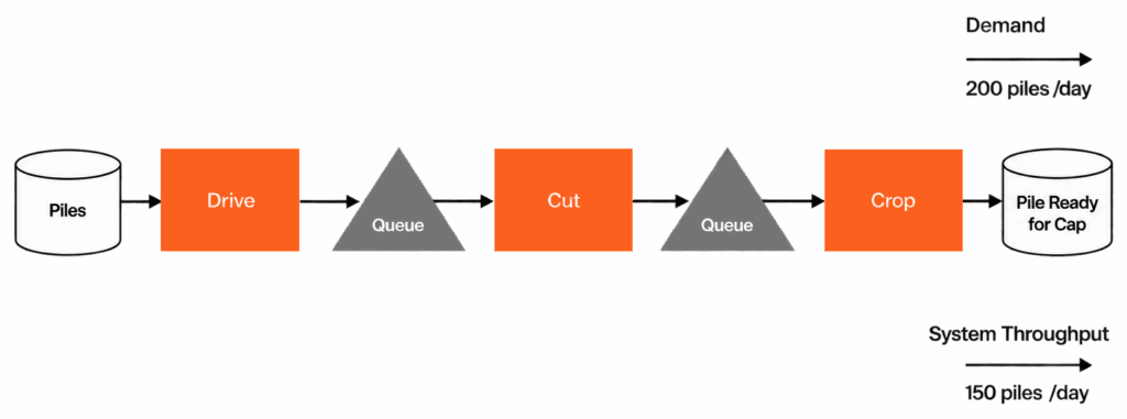
The term average is important because actual Throughput rarely remains constant. Production systems are subject to numerous sources of variability, including fluctuations in craft labor and knowledge worker productivity, equipment reliability, material availability, work quality, environmental conditions, and even management decisions. As a result, the number of units produced on any given day may differ from the number produced on the next. Throughput therefore fluctuates over time, even when the system is operating under seemingly similar conditions.
Satisfying Demand does not imply that Throughput will exactly match Demand at every point in time. Because production systems are inherently variable, daily or weekly Throughput will often fluctuate above and below the required Demand rate, and only if the system has the capacity to do so. The objective is therefore not to achieve a perfect mathematical match at every instant, but rather to design and control the system such that average Throughput reliably satisfies Demand over time. Throughput should not be confused with Capacity or Load as we expand next.
As shown in Figure 2, each operation in the production system is characterized by its own throughput rate, and the system itself has an overall throughput rate. Owing to variability in processing times, flow interruptions, and differences in operational capacities, the throughput of the overall system is generally not equal to the throughput of individual operations. Rather, system throughput emerges from the dynamic interaction among all operations and is primarily governed by bottleneck constraints and the propagation of variability across the production system.
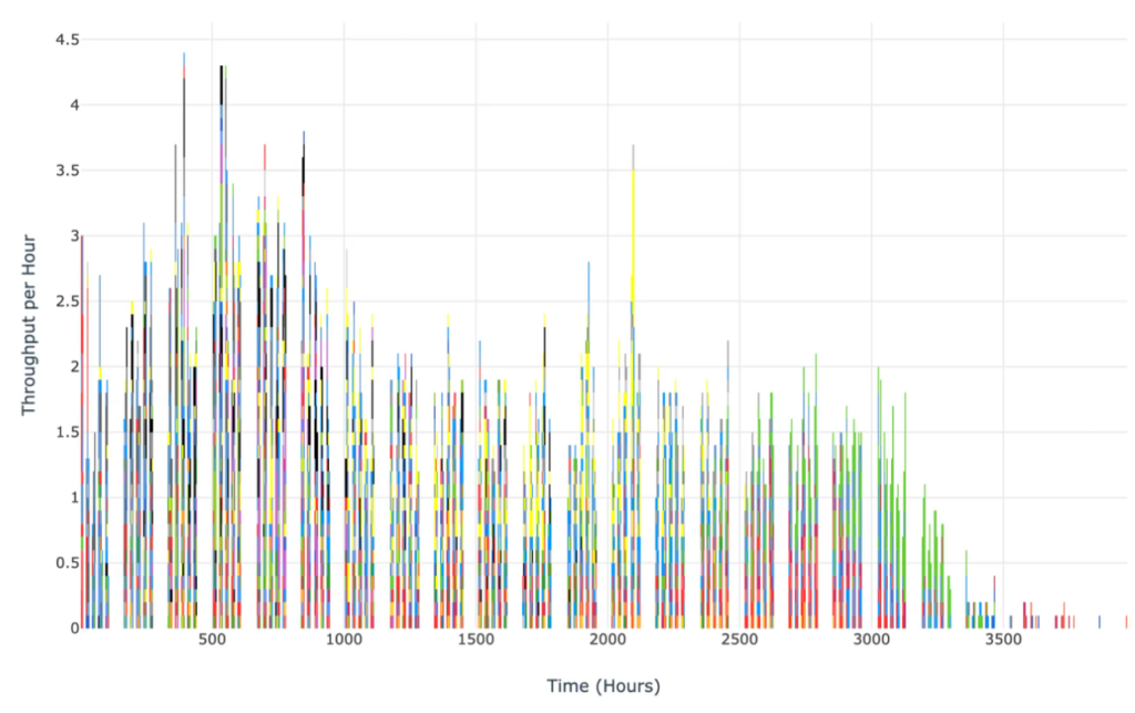
Figure 7 illustrates a Throughput chart example where the production system produces a certain volume of work at a given speed (Throughput per hour) and how it changes over time until production stops.
Capacity is the maximum sustainable throughput rate that a production system can achieve under specified operating conditions. As such, it is also measured as units over time. It represents the upper limit of Throughput and defines the maximum rate at which conforming units can be produced over time. In theory, a production system can only produce at Capacity when it operates without losses caused by variability, disruptions, quality defects, equipment failures, resource constraints, or other sources of performance degradation. In practice, however, variability is present in every production system, including project production systems, so operating sustainably at Capacity is not possible. To maintain capacity utilization levels that produce acceptable cycle times, production systems must operate below Capacity, leaving sufficient protective capacity to absorb variability.
This principle has important implications for production system design and control. As Throughput approaches Capacity, system utilization increases and the effects of variability become increasingly pronounced, resulting in longer queues, higher work-in-process levels, and longer cycle times. Consequently, attempting to operate continuously at Capacity often degrades overall system performance rather than improving it.
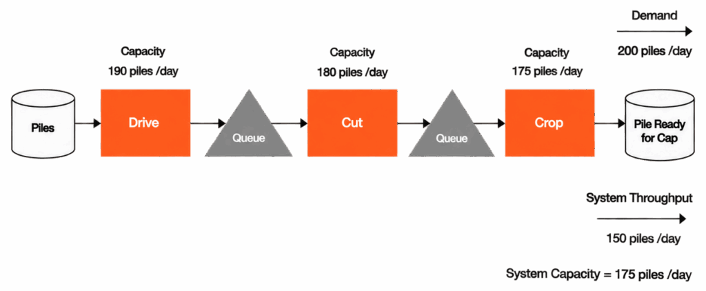
To determine the Capacity of a production system as per a given design or configuration, it is first necessary to identify the bottleneck. The bottleneck is the resource, process, or operation with the lowest effective Capacity (or higher Capacity Utilization), and therefore, establishes the maximum sustainable Throughput of the entire system. This rate, commonly referred to as the Bottleneck Rate (BNR), sets the pace of the production system because no production system can sustain Throughput greater than the Capacity of its bottleneck. As shown in Figure 2, each operation in the production system is characterized by its own capacity rate, and the system itself has an overall capacity rate.
Building on the previous piling production system example, the schematic below adds not only different capacity rates for each operation, but also for the overall system. Crop is the slowest operation so the system cannot produce more than 175 piles / day, and in this case, it cannot meet the demand. Because of variability, Throughput is lower than System Capacity and individual capacity rates.
This discussion brings us back to another important production system parameter: Capacity Utilization (CU). Unlike throughput or capacity, Capacity Utilization is not a rate; rather, it is a dimensionless measure, typically expressed as a percentage, that quantifies the extent to which available production capacity is required to satisfy demand. In this context, Capacity Utilization is defined as the ratio of Demand to Capacity. A Capacity Utilization of 100% indicates that the required Demand exactly matches the maximum sustainable Capacity of the production system. Values below 100% indicate the presence of excess capacity, whereas values above 100% indicate that the required Demand exceeds the system's available Capacity.
When Demand exceeds Capacity, as in the piling example presented above (CU = 200/175 × 100 = 114.3%), the production system is required to operate beyond its maximum sustainable output rate. Under such conditions, the system is unable to satisfy the required Demand, and a backlog of work will inevitably accumulate. Unless Capacity is increased, schedule performance will progressively deteriorate as the gap between required and achievable output continues to widen. If Demand is reduced, but Capacity not increased, schedule performance will also deteriorate.
For this reason, Capacity Utilization is a valuable metric for assessing whether available Capacity is sufficient to support planned project delivery rates. It also provides a direct measure of capacity buffers, which represent the portion of available Capacity not committed to meeting current Demand. For example, a resource operating at an average Capacity Utilization of 75% possesses, in average, a 25% capacity buffer that can be used to absorb production variability, accommodate demand fluctuations, or support increased production requirements without compromising system performance.
Load is a throughput rate that represents the amount of work assigned to, or required from, a specific operation within a production system. While Throughput is the average output rate achieved by the production system or operation, Load represents the output rate that the operation is expected to process to satisfy system demand. Although both Load and Throughput are expressed as rates and provide insight into system performance, it is important to distinguish between them. Due to variability, resource constraints, and other operational factors, the actual Throughput achieved by an operation may differ from its Load. Consequently, increasing the Load imposed on an operation does not necessarily result in a corresponding increase in Throughput. For this reason, Load, Throughput, and Capacity should be viewed as distinct production system parameters, each describing a different aspect of system behavior.
For a given operation, Load may equal Capacity. In such a case, Capacity Utilization is 100%, as Capacity Utilization can be calculated as (Load / Capacity) × 100%. When Capacity Utilization reaches 100%, the operation is fully loaded and has no remaining capacity buffer. Under these conditions, the operation lacks the ability to absorb variability, disruptions, or increases in demand without negatively affecting performance. As a result, even minor fluctuations in processing times or work arrivals can lead to queue formation, increased cycle times, and reduced system reliability.
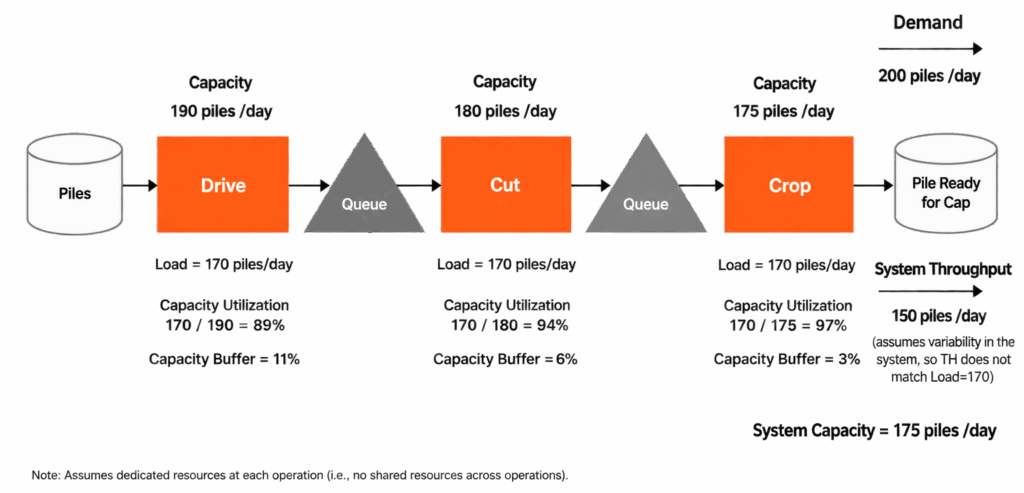
Building on the piling production system example introduced previously, Figure 9 incorporates the concept of Load. For illustrative purposes, a Load of 170 piles per day is assumed for the Drive, Cut, and Crop operations (Load could also be set to match the capacity of each operation). Because the Capacity of each operation differs, the resulting Capacity Utilization levels also differ. Under these conditions, Drive operates at 89% Capacity Utilization, Cut at 94%, and Crop at 97%. Since the Crop operation exhibits the highest Capacity Utilization, it possesses the smallest capacity buffer and is therefore the bottleneck of the production system. As the operation working closest to its maximum sustainable Capacity, Crop is the most vulnerable to the effects of variability and is the first operation likely to constrain overall system Throughput. Consequently, the performance of the entire production system is largely governed by the ability of the Crop operation to sustain the required Load.
Rework represents the portion of completed output that fails to meet specified requirements and must re-enter the production system for correction, at some specific point in the system, before it can be accepted as finished work. Unlike Demand, Throughput, Capacity, and Load, which are measured in units / time, Rework is typically expressed as a percentage of output.
Because Rework is common in engineering and construction, it is present in many project production systems. However, Rework is not an inherent characteristic of all production systems, as some processes may consistently produce output that meets requirements without requiring correction or repetition of work. For this reason, Rework differs from Demand, Throughput, Capacity, and Load, which are fundamental parameters present in every project production system. Rework induces an additional flow of work generated when previously completed output fails to meet specified requirements and must be corrected or modified.
Although not always present, Rework can have a significant impact on system performance because it consumes capacity, increases work-in-process, extends cycle times, and reduces the capacity available to produce new outputs. As a result, even relatively low levels of rework can substantially affect the throughput and overall performance of a project production system.
Rework can be experienced in engineering and design, fabrication, assembly, testing, installation, commissioning, maintenance, and even decommissioning of assets. But regardless of the production context, a Rework ratio quantifies the fraction of work that requires additional processing, which increases the Load imposed on an operation or system. As Rework levels increase, additional Capacity is consumed to correct previously completed work, which can reduce system Throughput, increase Capacity Utilization, lengthen cycle times, and adversely affect schedule performance. Minimizing Rework is therefore essential for maintaining the flow of production, preserving capacity buffers, and achieving stable and predictable production rates.
Building on the piling production system example introduced previously, Figure 10 incorporates the concept of Rework. Although Rework may also occur at the Drive and Crop operations, this example assumes that Rework occurs only at Cut and is equal to 20% of the output rate. Prior to accounting for Rework, the Cut operation was loaded at 170 piles per day. With a Rework rate of 20%, 34 piles per day fail to meet requirements and must re-enter the Cut operation for correction. As a result, the effective Load on Cut increases from 170 piles per day to 204 piles per day. However, what Crop receives is limited by Cut’s capacity.
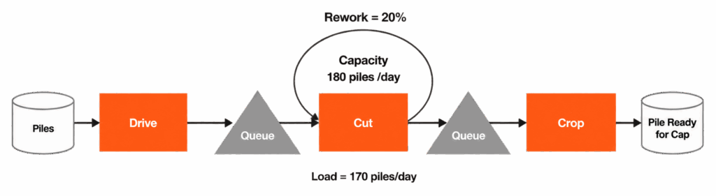
This increase in Load has a direct effect on Capacity Utilization. Previously, the Capacity Utilization of Cut was 94%, calculated as 170/180. After accounting for Rework, and assuming capacity remains the same, Capacity Utilization increases to 113%, calculated as 204/180. Therefore, the Cut operation is now being required to process more work than its available Capacity can sustainably support. Consequently, the presence of Rework at Cut has changed the behavior of the production system. While Cut was not previously the bottleneck, the additional Load created by Rework causes its Capacity Utilization to exceed 100%, making Cut the new system bottleneck. Under these conditions, the operation cannot maintain the required production rate, and WIP will accumulate unless Rework is reduced, additional Capacity is added, or Load is otherwise reduced.
Scrap represents the portion of completed output that fails to meet specified requirements and, due to its condition or the cost of recovery, cannot be reworked and returned to the production system to become acceptable finished work. Unlike Rework, which creates additional Load by requiring corrective processing, Scrap results in a permanent loss of productive output and the resources that were consumed to create it. Scrap loss reduces the Load on downstream processes.
Although the term Scrap is most associated with physical production processes such as fabrication, assembly, and installation, it can also occur in non-physical work processes. In engineering and design, for example, completed work products may become obsolete, invalid, or unusable due to errors, changes in requirements, or superseding design decisions. In such cases, the effort invested in producing the work is effectively lost and must be replaced with new work.
From a production perspective, Scrap reduces the efficiency with which Capacity is converted into acceptable output. Resources are allocated and used to produce work that ultimately generates no value toward project completion, thereby reducing effective Throughput. As Scrap levels increase, additional Capacity is required to replace the discarded output and maintain the desired delivery rate. Consequently, high Scrap ratios can increase Capacity Utilization, consume capacity buffers, and negatively affect schedule performance. For this reason, minimizing Scrap is essential for preserving production system efficiency and maximizing the proportion of Capacity devoted to generating acceptable finished work.
Building on the piling production system example introduced previously, Figure 11 incorporates the concept of Scrap at the Drive operation and assumes a Scrap ratio equal to 30% of the output rate. Prior to accounting for Scrap, the Drive operation was loaded to produce 170 piles per day. With a Scrap ratio of 30%, 51 piles per day fail to meet requirements and must be discarded, leaving only 119 acceptable piles per day available for release to downstream operations. As a result, the effective Throughput of the Drive operation is reduced from 170 piles per day to 119 piles per day. In other words, although Drive expends the Capacity required to produce 170 piles per day, only 119 piles per day contribute to overall system throughput. The Capacity consumed to produce the scrapped piles is effectively lost.
It should be noted that the value of 119 piles per day represents the expected Throughput based on the average Scrap ratio. In practice, production systems and their operations are subject to variability in processing times, operating conditions, and quality performance, therefore, the actual Throughput achieved by the Drive operation may fluctuate and fall below 119 piles per day.
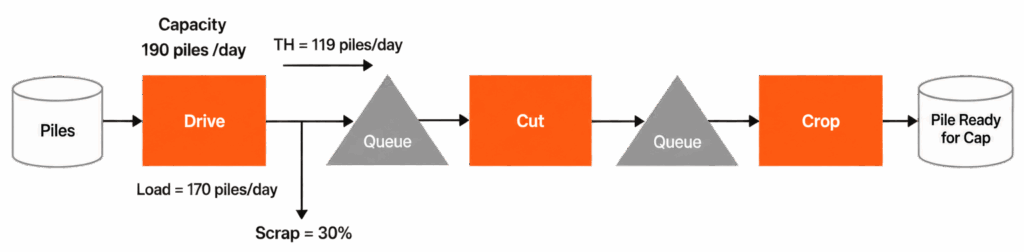
This example illustrates the significant impact that Scrap can have on production system performance. Unlike Rework, which increases Load by requiring additional processing, Scrap directly reduces effective Throughput by eliminating a portion of the completed output. Unless Scrap ratios are reduced or additional Capacity is provided, the resulting loss of Throughput can constrain downstream operations, reduce overall system performance, and adversely affect production rates, and therefore, schedule dates.
This paper has introduced fundamental production measurements that characterize the flow of work through project production systems: Demand, Capacity, Throughput, Load, Rework, and Scrap. Together with WIP and CU, these measurements provide a practical Operations Science framework for understanding, designing, controlling, and improving project production systems. While production rates describe how work enters, flows through, exits, and re-enters a production system, WIP and CU define important operating conditions that influence Throughput, Cycle Time, queue formation, responsiveness to variability, and ultimately project performance.
The engineering and construction industry has long relied on measurements associated with project administration and management, including labor rates, equipment rates, billing rates, cost expenditure rates, and other metrics like time on tools, productivity factors, and takt. While these measures are important for planning, reporting, and controls, they do not explain how work flows through the production systems responsible for delivering project outcomes. The measurements presented in this paper belong to a different category. They describe the behavior of the systems that use resources to transform requirements, information, and materials into deliverables and completed assets.
Viewed through this lens, projects are not merely collections of activities linked by a schedule. They are networks of interconnected production systems. The performance of these systems is determined not only by the work they perform, but also by the rates at which work enters, flows through, exits, and re-enters the system. Understanding production measurements therefore provides a more direct means of explaining, predicting, and improving project performance than relying solely on administrative or financial measures.
Perhaps most importantly, these production measurements, including rates, ratios and various operating parameters, should not be viewed independently. Demand establishes the production requirements imposed on the system. Capacity defines the maximum sustainable output that the system can achieve. Load determines the amount of work imposed on individual operations. Throughput reflects the output actually produced, while Rework and Scrap consume Capacity without directly contributing to project objectives. WIP determines how much work resides within the system at any point in time and can be directly influenced through production control policies. Capacity Utilization defines the operating point of the production system and can be intentionally designed by balancing the Load imposed on the system with its available Capacity. Together, these measures determine how efficiently work flows through the production system, how resilient it is to variability, and whether it can reliably satisfy project Demand.
As you evaluate the production systems within your projects, consider the following questions:
The answers to these questions provide far more than a snapshot of project performance. They reveal how the production systems responsible for delivering the project are designed, how they are operating, where constraints and losses exist, and where opportunities for improvement can be found. By understanding and managing the relationships among production rates, ratios, WIP, and Capacity Utilization, project teams move beyond monitoring project outcomes to actively designing and controlling the production systems that create those outcomes. In doing so, they gain the ability not only to explain project performance after it occurs, but also to predict, influence, and improve it before it occurs.
Ultimately, project performance is not created by schedules, budgets, or management reports - it emerges from the behavior of production systems. Understanding and managing production rates and measurements including WIP and Capacity Utilization, provides project professionals with a practical Operations Science framework for designing, controlling, and continuously improving those systems.