Herein we describe a refinement of the well-known Cycle Time Formula, introducing two new components into the formula. One component describes the “wait-to-match” time of different routings in a production system converging at a single point, such as in an assembly operation. The second component accounts for “planned time buffers” – the time that parts or tasks are waiting, whether or not they can be worked on because of policies governing whether work can be done or not. Including these new components leads to a deeper understanding of the key contributors to cycle time, allowing us to make better decisions to optimize production system performance for considerations such as time-to-market or minimizing cash tied-up in Work in Process (WIP).
Keywords: Cycle Time; Wait-to-Match; Planned Time Buffer; Work in Process
As the Operations Science framework continues to be applied to understand and optimize production systems, both in project and manufacturing environments, the framework itself may be refined to better describe the behavior of a production system. One such example is the components of cycle time, as described in this article.
Before we begin, it is critical to note that in numerous Project Production Institute (PPI) papers and presentations, we’ve conveyed the notion that cycle time is a lagging indicator, whereas Work-In-Process (WIP) is a leading indicator for a production system, and the relationship between the two is clearly described in Little’s Law. So, why do we have to better understand what constitutes cycle time when we can just control WIP?
It is because the optimal amount of WIP to maintain a production system is not arbitrarily chosen by picking a number from thin air, but rather determined by the design of the system, including policies that govern its behavior such as operations sequence, types and numbers of equipment used, process batch, transfer batch, work schedules, control type (push, pull, CONWIP), etc. Therefore, it is critical to understand what is driving cycle time to increase or decrease, if factors such as the amount of cash tied-up or time-to-market are of concern. To achieve this, let’s examine the definition and components of cycle time.
Per the PPI Glossary [1], Cycle Time is defined as “the average time from when a job is released into a station or line to when it exits,” whereas Process Time is defined as “the time a job spends at an individual station in a production system from the time the station begins working on it, until the time the station finishes.” In most real-life production systems, if not all, Cycle Time is greater than Process Time due to an item “waiting” to be processed. Although capacity can wait for an item to arrive, this is not considered part of the cycle time, it doesn’t increase the overall time for the item.
Since the downtime of capacity is calculated as part of the effective process time, the resulting cycle time can be formulated as follows:
CT = RPT + BT + MT + QT + SDT + WTMT + PTB
Some of these components have been described in many previous papers and presentations. These are:
Raw Process Time (RPT): The sum of average time required to process a single transfer batch including all detractors such as downtime and setup time (RPT = PT + ST + DT). It does not include queue time or the time blocked when a downstream station has no queue space
Process Time (PT): The time a job spends at an individual station in a production system from the time the station begins working on it, until the time the station finishes
Setup Time (ST): The time required to go from the end of the last good part from one batch to when the first good part of the following batch is produced
Downtime (DT): The time during which a machine, especially a computer, is out of action or unavailable for use
Batch Time (BT): The time jobs spend waiting due to batching and is composed of Wait-to-Batch Time and Wait-in-Batch Time. Waitto-Batch Time is the time jobs spend waiting to form a batch for either (simultaneous) processing or moving. Waitin-Batch Time is the average time a part spends in a (process) batch waiting its turn on a machine
Move Time (MT): The time jobs in a production system spend being moved from one station in the production system to the next station, including the time waiting to move. This definition of move time assumes a resource is always available to move the job (i.e., not capacity constrained).
Queue Time (QT): The time that parts or tasks spend waiting for processing at a station or to be moved to the next station (if move resources are capacity constrained). Using Kingman’s Equation [2], which describes the factors that determine the QT, it can clearly be seen that increasing utilization as well as increasing variability both result in greater queue time.
Shift Differential Time (SDT): The time that parts or tasks spend waiting for processing or to be moved due to different resources working on different schedules (e.g., the first resource works 24 hours per day while the second only works 16 which results in an average of 4 hours of SDT).
However, this paper introduces two new components of cycle time to make sure all categories of waiting are included:
Wait-to-Match Time (WTMT): The time that parts or tasks spend waiting for its counterpart at an assembly operation
Planned Time Buffer (PTB): The time that parts or tasks spend waiting due to policies that govern whether work can be done or not
Let’s examine these two new components in more detail.
For Wait-to-Match Time, let’s consider a production system where multiple flows come together as input to the subsequent flow (Figure 1). In this case, there is always a chance that output from one of the flows will wait for output from another in order to start the subsequent flow – this is known as “wait-to-match”. It can happen even if all flows have a batch size of one. Therefore, the “Wait-to-Match” time component has been singled out as an independent item distinct from and not a part of the Batch Time as previously considered.
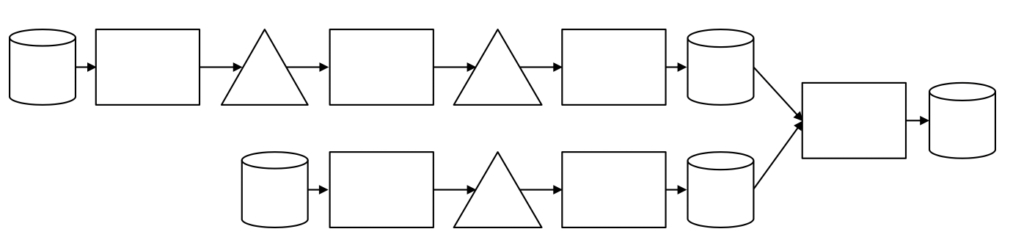
Figure 1. Example of Assembly Process with two flows converging to a single flow
Planned Time Buffer, although not considered explicitly in the original cycle time formula, has been described by PPI for such use, as well as in many documents and presentations by the industry. It is typically introduced as a means to protect capacity from low utilization (e.g., Era 1 thinking [3]). Some examples are: ensuring materials are onsite six weeks before usage, placing an order x months before the lead time quoted by the supplier to ensure on-time or early delivery, not starting work although all material and equipment is ready since schedule says not to, etc. In essence, providing a Planned Time Buffer is the same as planning for a stock. Little’s Law shows that for a given throughput (i.e. the lesser of the demand or the capacity of the line), TH, the average resulting stock, S, will be:
S = TH x PT
Although some of these policies may have a solid basis, the resulting stock may be an equal or greater risk for the entire production system. Moreover, when setting a PTB, people usually do not employ optimal (or even near-optimal) stocking policies, often resulting in much larger stocks than needed to ensure scheduled starting times.
However, regardless whether an item is in WIP or Stock, they all are considered inventory, which is cash tied-up in the system (Figure 2). If there is an amount of cash tied up in the system, or if the cycle time is of concern, then careful consideration must be taken in order to ensure that the management decision is not just trading one component of cycle time for another, e.g., building up stocks in order to reduce the process time of subsequent operations only to have the output wait (queued) for the next operation. Another example of mismanagement is increasing batch size to reduce the setup time only to have the batch time increase offset the gains made by increasing the batch. Since it is possible to calculate these trade-offs, they should not be determined by trial-and-error, but rather optimized by using basic Operations Science relationships.
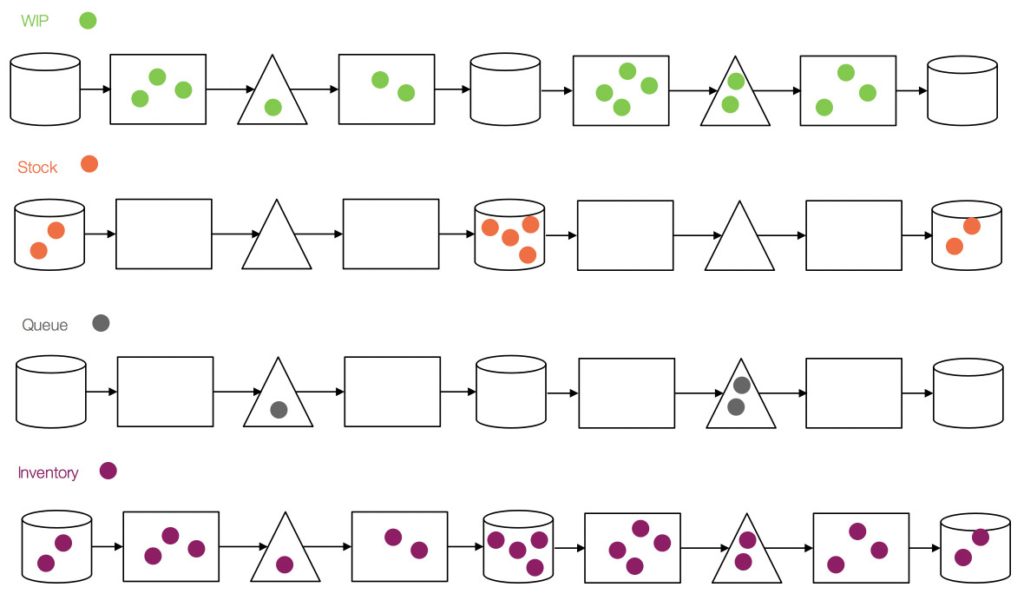
Figure 2. Types of Inventory
If the amount of cash tied-up or time-to-market is of concern in a project, it is critical to understand what components of cycle time cause it to increase or decrease. This paper has revisited the cycle time formula to better capture the contribution of two components – planned time buffers and the amount of time waiting for a match. By having a clear understanding of all cycle time components, it is possible to calculate trade-offs between them using basic Operations Science relationships rather than using trial-and-error.