Application of Operations Science to Design a Project Production System: A Case Study in Building Construction

Introduction

A common practice in delivering construction projects (or simply ‘projects’) is to use “conventional project management” (simply ‘PM’) as a body of management knowledge [1]. However, this body of knowledge lacks two fundamental concepts that are useful in delivering projects, as Shenoy & Zabelle [2] pointed out. First, conventional project management practices focus on planning and forecasting, but ignore that production occurs throughout the project thus overlooking the need to organize detailed work activities, resources that perform the work, and inventories that determine the actual duration of the work and thus affects overall project performance. Second, these practices do not offer a technical perspective and the tools to effectively manage variability and inventory (stocks and work-in-process), yet variability and inventory are interdependent and together drive overall project performance.

One way to address these technical and performance gaps is to apply production system design (PSD), including system optimization, either before or while the production system is operational. “PSD is concerned with the development of operation and process design in alignment with product design, the structure of supply chains, and the allocation of resources [3].” It can involve the implementation of lean concepts, such as pull production, batch sizing, the use of takt time, and buffering [4], [5], [6], [7]. As a part of the PSD process, OS can be used for system optimization. This requires the collection of production-related data as input for models that can help to gauge the system’s performance. However, due to limitations of conventional construction management practices (e.g., lacking production-related metrics and data to gauge performance) and characteristics of construction systems (e.g., these systems seldom operate in a steady state), conducting an OS analysis is challenging.

With this in mind, the purpose of this paper is to demonstrate the applicability of conducting an OS analysis based on the PSD of a case-study project, namely the construction of a healthcare building in Northern California. The paper starts by summarizing literature about PSD and OS applied to projects in the construction industry. Then, the research method section presents the steps followed in this study. The case study and discussion sections present the OS analysis. This paper ends with conclusions and recommendations for future research.

Litreature Review

PSD has seen widespread application in manufacturing. Skinner [8] stated that the PSD objective is to determine a set of policies in the manufacturing setup, and these fall into two groups. The first group is related to resource capacity, facilities, equipment, and technologies to use. The second group is related to infrastructure, workforce management, production planning, and control. According to Askin & Goldberg [9] PSD is about managing production resources to meet the customer’s demand. CIRP (Collège International pour la Recherche en Productique, French acronym of International Academy for Production Engineering) [10] defined PSD as the conception and planning of the overall set of elements and events constituting a system, along with the rules for their relationships in time and space. PSD involves (1) defining the problem(s) and objective(s), (2) outlining the alternative streams of action, (3) evaluating those alternatives, and (4) developing the detailed design of proposed production systems. The result of the PSD, whether achieved by creating a new system or changing an existing one [11], is a description of the production system [12].

The applicability of PSD in the construction industry has been recognized for at least 30 years. Koskela [13] stated the need for implementing a new philosophy of production to construction based on just-in-time (JIT) production and quality management as implemented by Toyota. Previous studies analyzed the application of discrete event simulation (DES) to illustrate the behavior of production systems in construction. For example, Tommelein [14] modeled the pipe-spool design, fabrication, and installation process using the STROBOSCOPE software [15] to show how project performance is affected by the manifestation of variability, specifically how the use of planning with push vs. pull-driven sequencing affects inventories and the project duration. She defined the “matching problem” (where unique parts need to be installed in uniquely designated areas) and demonstrated its potential impact on project performance. Indeed, the matching problem becomes visible at the level of production planning but in conventional project management is ignored at the project planning level. Tommelein [16] also mentioned that the increased use of standard products in construction could alleviate matching problems.

Ballard & Howell [17] stated that “construction is essentially the design and assembly of objects in a fixed position and consequently possesses, more or less, the characteristics of site production, unique product, and temporary teams.” Especially fixed position onsite construction (without consideration of supply networks, e.g., of the production of preassemblies and modules) provides limited opportunity to outright apply manufacturing production methods. Nevertheless, Ballard et al. [3] presented a guideline for PSD in construction projects, acknowledging the need for allowing tradeoffs between goals in a project and the conception of a “project-based production system” as the type of production system in construction. Following these ideas, Koskela & Ballard [18] developed a three-level requirements hierarchy framework for PSDs in construction that recognizes the need for using Operations Management (OM) concepts.

At the same time, researchers studied Lean Construction tools and methods to use in PSD. The following references are but a few of many applying such tools and methods. Schramm et al. [19] used the line of balance (LOB) method to plan low-income housing projects, concluding that it was crucial to consider the whole production system rather than individual activities. Kemmer et al. [20] used the LOB to communicate concepts related to production management, such as cycle time (CT) and work-in-process (WIP) metrics. Schramm et al. [21] showed how PSD can support the adoption of a customization strategy in housing projects, improving transparency and predictability. Murguia & Urbina [22] used Building Information Modeling (BIM) 4D models for PSD of non-linear and non-repetitive construction processes. Barth et al. [23] implemented PSD with BIM in the Chilean house building sector to improve plan accuracy and logistics planning using production-related metrics, including CT, WIP, and takt time.

Various applications of PSD in the construction industry have demonstrated how production systems can achieve various levels of project performance. Nonetheless, knowledge appears to be lacking about how PSD can affect project performance. Knowledge about OS provides a foundation for applying manufacturing concepts related to PSD to the construction industry. When applied to manufacturing, OS is called Factory Physics [24], [25]. When applied to projects, it is called Project Production Management (PPM). PPM is viewed as the delivery model for the 3rd era of project delivery [2].

OS is rooted in OM and Operations Research (OR). OM pertains to managing processes and operations that produce goods and services [26]. Adam [27] organized various points of view on OM (e.g., management science, the systems view, the managerial process approach) and found that, depending on the point of view, practitioners apply OM differently. Swamidass [28] recognized the need to broadly consider all topics related to OM and suggested that building an empirical theory for OM might provide substantial benefits to practitioners interested in applying OM.

OR pertains to systematic approaches for formulating and solving problems using mathematics and analytical tools in the process of analysis [29]. These approaches can be applied to different problems in various disciplines and industries [30]. Heiman [31] explored the use of OR in the construction industry, concluding that OR may examine problems to seek causes rather than treat effects. From early on OR has been used in construction to solve scheduling problems. Despite some overlap in their uses and methods, Fuller [32] pointed out that “At the conceptual or philosophical level, OM and OR differ substantially. OM is concerned with managing production resources critical to a company or organization’s strategic growth and competitiveness. It entails designing, operating, controlling, and updating systems responsible for the productive use of human resources, equipment, and facilities in developing a product or service [33].”

Considering the need for an empirical theory of OM [28] and the development of OR as a science [30], Hopp & Spearman [24] proposes a “science of the operations” (OS). OS is the study of the transformation of resources to create and distribute goods and services [34]. It focuses on the interaction between demand and production (supply) and the variability associated with either or both. OS also describes the set of buffers required to synchronize demand with production [35]. OS is the science that describes the behavior of operations [36]. Shenoy [37] compared OM, OR, and OS. He noted that OR describes the mathematical and analytical techniques used to make better decisions in OM. Furthermore, OS uses principles and equations to unify the concepts of OM and OR, applicable not only to manufacturing but to any production system (including construction projects). Among other authors, Prado [38] described their applicability to offsite construction projects to accomplish a JIT delivery and production control.

Considering all the benefits of applying OS-related concepts, it is essential to acknowledge that even though “projects are different,” the manufacturing industry provides the elements to construct buildings, bridges, highways, and factories [39]. Therefore, the application of OS to the project, including engineering, manufacturing, supply, installation, assembly, and commissioning can enhance the entire project production system. The questions this study is trying to address are: How can an OS analysis inform the PSD of a construction project? and What assumptions must be made to conduct such an analysis?

Research Methodology

The research methodology selected to demonstrate the applicability of OS to PSD includes the use of analytical modeling capabilities within Production Optimizer (proprietary software provided by Strategic Project Solutions Inc.), which has discrete event simulation capability (DES) as well and the use of some of the three equations and four performance graphs described in Factory Physics [24]. We obtained production data describing a case study project, namely the cladding installation process of a healthcare building in Northern California.

This study makes use of four interrelated OS metrics to explain the behavior of project production systems, defined as follows (also see [40]):

1. Cycle time (CT): CT is the time it takes a product, piece of information, or chunk of work (e.g., a room or building) to go from the beginning to the end of a production process; that is, the time it is WIP. It is the time for a product to transit the system, thus defined by how one defines the boundaries for that system.
2. Work-in-process (WIP): WIP consists of inventory between the start and end points of a routing.
3. Throughput (TH): TH is measured as the average output of a production process (machine, station, line, plant) per unit of time.
4. Capacity utilization (u): u is the percentage of a resource’s capacity that is used in production.

This study makes use of the following equations and graphs [24]:

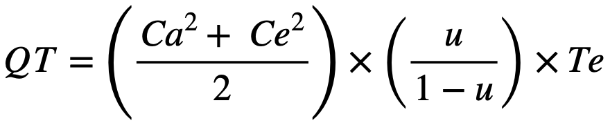
The Variability, Utilization, and Time (VUT) Equation: The VUT equation (also known as the Kingman equation) is an approximation for the mean waiting time in a queue in a system with a single server where arrival times have a general (meaning arbitrary) distribution and service times have a (different) general distribution [35]. Equation 1 shows the industrial engineering version of the Kingman equation, where Ca2 is the squared coefficient of variation of interarrival times, an indicator of demand or flow variability; Ce2 is the squared coefficient of variation of effective process times, an indicator of process variability; Te is the mean process time.; and u is the utilization. u has a significant impact on QT, as explained by Roser [41] and others; the higher u, the more prolonged QT, which will approach infinite as u reaches 100%.

Little’s Law: Describes the relationship between WIP, CT, and TH for production flows (equation 2). From a practical standpoint, this means that WIP is a leading indicator of CT. Among other authors, Gharaie et al. [42] applied Little’s Law to the house-building industry.

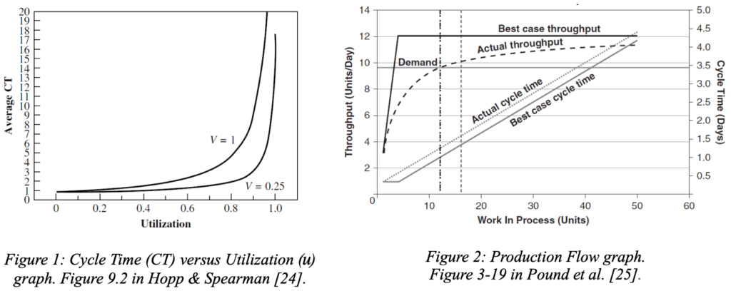
Cycle Time versus Utilization graph: This graph shows that when capacity utilization (u) increases toward 100 %, queue time (QT), which is a component of CT, increases toward infinity. As shown in Figure 1, with more variability (comparing curve V=0.25 and curve V=1, where V represents the amount of variability in each curve), the CT tends to go to infinity more quickly when u has a higher value. This graph represents the combined effect of u and variability on CT, showing that it is necessary to control both when trying to optimize a CT.

Production Flow graph: The Production Flow graph (Figure 2) actually combines two graphs: TH versus WIP and CT versus WIP. It shows that an increased amount of variability in the production system causes deterioration in performance, with the actual throughput curve falling below the best-case throughput curve (the best case corresponds to zero variability). Similarly, it causes the Actual cycle time curve to increase above the best-case cycle time curve. Given a production system’s capacity and variability level, CT and TH vary directly with the amount of WIP in a system. Therefore, WIP is a design and control parameter for determining the amount of TH and CT.

Case Study: Construction of a Healthcare Building in Northern California

The case study pertains to a $158 million investment to expand the Sutter Santa Rosa Regional Hospital (SSRRH) and increase its capacity [43]. The SSRRH project consists of a new three-story expansion wing on the east side of the hospital, tied to an existing hospital structure on the 1st and 2nd floors. The expansion adds 58,000 square feet of space and includes forty patient beds in all-private rooms, one endoscopy and gastroenterology room, twenty intensive care unit beds, and eleven post-anesthesia care unit bays [44]. The project owner was Sutter Health, the architect was Stantec, and the construction manager and general contractor was the Herrero-Boldt joint venture. The project applied an Integrated Project Delivery (IPD) arrangement with commercial terms spelled out in an Integrated Form of Agreement (IFOA) [45]. This hospital expansion project is the first of this kind regulated at the state level by the Department of Health Care Access and Information (HCAI) to use an offsite, panelized exterior skin (cladding system) (HCAI healthcare building type 1). The project was delivered successfully, saving almost $800,000 relative to the initial budget and shaving off four months from an already tight schedule. The delivery project team received several awards for their success, including for the use of their innovative cladding system. We selected the cladding system construction process to apply OS to PSD. The study included the cladding system’s installation (onsite assembly) process with its engineer-to-order (ETO) components, specifically Exterior Insulation and Finish System (EIFS) panels.

The authors conducted interviews and led workshops to collect data from the project staff. This data helped to define the parameters of the production system, which are process batch (PB, also called current reorder quantity), transfer batch (TB), and demand (D) of each of the steps considered in the construction process to analyze. Other data, such as the number of completed activities in a day, was needed because it provides a rate at which the construction crews perform the work. This rate provides an idea of the process rate (PR) or process time (PT) by dividing the number of completed activities or units in a full day (or on an hourly basis). Furthermore, data was needed about the number of resources used in each of the construction process activities. The resources can be a combination of people, materials, pieces of construction equipment, subcontractors, and services required. The data about the resources helped to quantify their capacity utilization based on the time available for the specific construction process. Data was also needed about the arrival time when work goes from one step to another.

Recognizing an OS application is stochastic in nature, we used the mean and squared coefficient of variation (SCV) of the data collected to represent variability in this construction process. More detailed information about the data collection process followed in this study can be found in Prado’s master’s thesis [46].

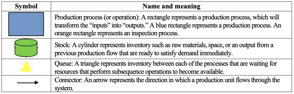
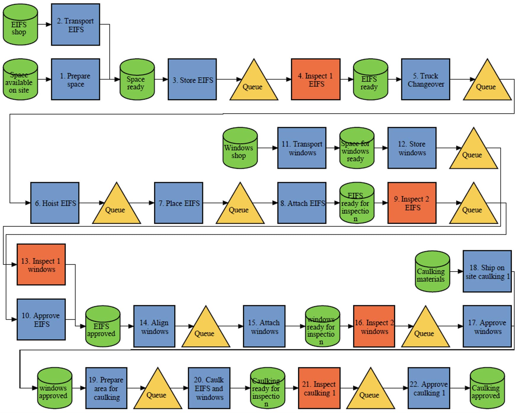
Based on the data collected, the authors used production process maps to expose the interactions between the stakeholders involved in the production system. Table 1 explains the symbols used. Figure 3 shows a map, that was created using the Project Production Institute´s (PPI´s) Process Mapper tool [47]; Considering this map and the data gathered from the project team, we developed an analytical model using the SPS Production Optimizer. The Production Optimizer implements an optimization algorithm based on OS metrics and equations combined with heuristics, and then produces graphs to depict a production system’s behavior.

The following assumptions were made to develop the OS model of this construction process:

1. The Production Optimizer uses a parameter named SCV, a normalized measure of variability in the system. According to the heuristics of SPS engineers, SCV = 0.5 reflects low variability, SCV = 1.0 medium variability, and SCV = 1.5 high variability. The SSRRH model is based on the value SCV = 1.5 to replicate a highly variable scenario.
   • If PR and PT are normally distributed parameters, then the SCV in the Production Optimizer is a relatively accurate variability metric. These parameters are assumed to have a normal distribution in the SSRRH model.
2. The Production Optimizer assumes that the system being modeled is in a steady state mode, i.e., the model has no “warm-up” phase.
   • In the case of the SSRRH model and in many construction projects more generally, a warm-up phase can be observed. For example, when starting a new operation crews need to figure out how they can work efficiently given the context they are working in. This warm-up may take a few days or more before a more-or-less steady state can be reached.
3. The Production Optimizer can account for a Wait-to-Match time in its analytical model; however, it does not capture unique matching [14] of parts.
   • It is assumed that the matching problem was addressed through impeccable coordination between the SSRRH project team members before the start of construction. It may therefore be reasonable to assume that no matching problems would arise.
4. Rework is not considered in the model.
   • The SSRRH project experienced almost no rework in their operations, thanks to the impeccable coordination as described in point 4 and the dry runs the team members performed.
5. There is no multi-tasking for resources or pre-emption of activities. The resources are working one step at a time. Once they start working on a product (or material) they complete all successive steps in that product’s flow between stocks before starting on a second product.
   • The SSRRH project team told us that the nature of their operations was to indeed to complete one sequence of activities prior to going to the next one, which resembles no shared resources between processes.

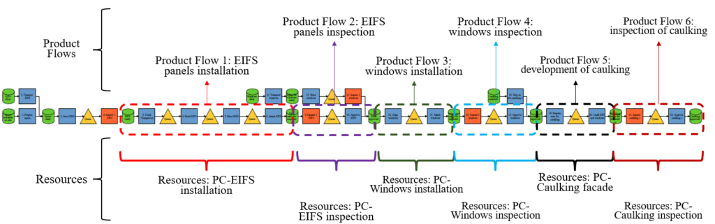
Figure 4 shows the allocation of product flows and resources in the production system process map. Each product flow corresponds to a resource (also called “process center” in Production Optimizer). The results sheet of Production Optimizer provides OS metrics and graphs for each pair of product flow and resource. In the model, we included the production-related parameters related to operations (PR or PT) and items (PB, TB, D).

The scope of this case study included the use of Little’s Law and the Capacity Utilization graph to describe the behavior of CT, TH, WIP, and u of the resources involved. Figure 5 shows the data we extracted from the results sheets of the Production Optimizer based on the OS analysis applied to each product flow. We used the Production Flow and Capacity Utilization graphs only to see the behavior of the OS metrics involved.

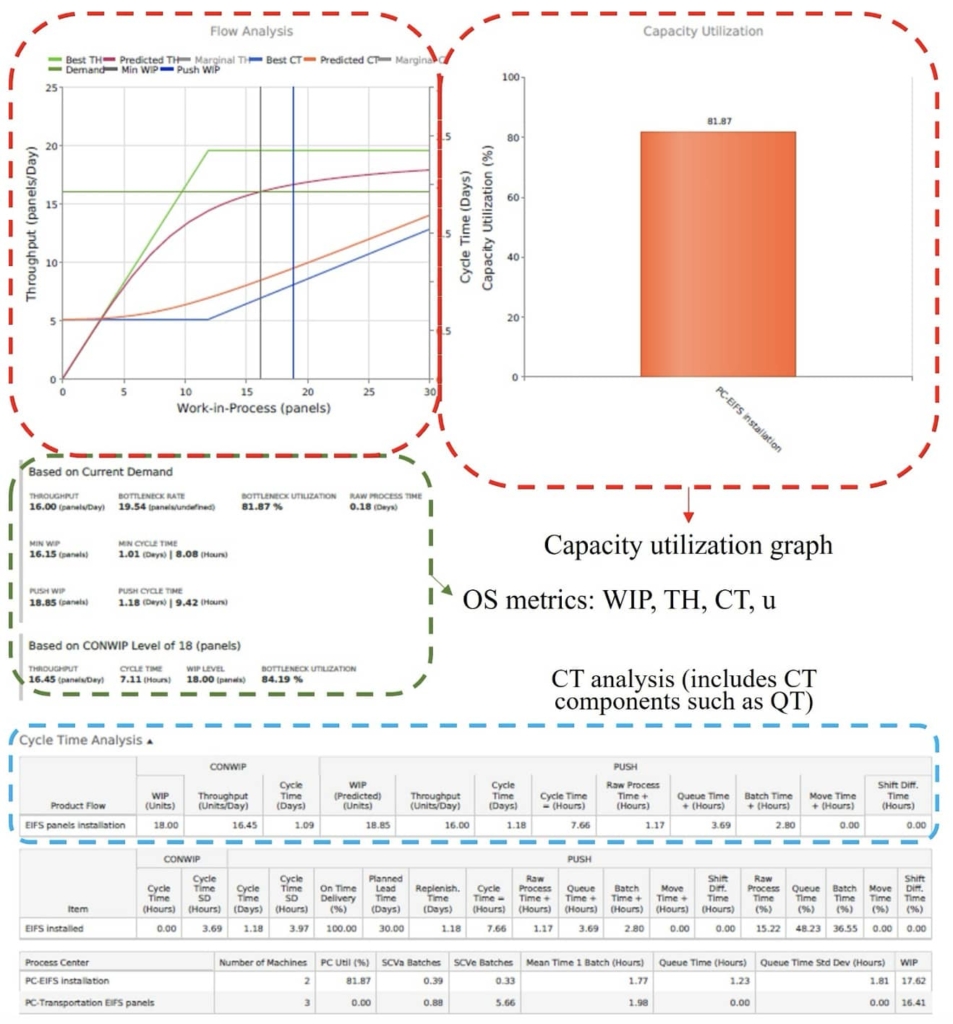
The Production Flow graph section of Figure 5 shows the TH of the production system, which can produce more than 16 EIFS panels/day (D). The project team initially established this D, and the analytical model’s results showed that the production system was able to satisfy this D. The intersection between the “Demand” and the “Predicted TH” (which considers the effect on variability in the TH) lines provides the “MINWIP” vertical line. MINWIP shows the minimum amount of WIP required to satisfy D. Similarly, the software algorithm in the Production Optimizer calculated the vertical line “Push WIP,” which shows the amount of WIP that works under a push production system.

The OS metrics section of Figure 5 also shows the results (TH, WIP, CT, u) with a CONWIP, if established for that specific product flow. Ideally, the CONWIP established to control the production system should be between these MINWIP and Push WIP vertical lines. In the case of the EIFS panels installation, the CONWIP can be between 17 to 19 EIFS panels to control WIP in the system and still satisfy the demand. Regarding the CT, Figure 5 shows that increasing the WIP of the system also increases the CT (“Predicted CT” line) to produce that specific TB. This is the tradeoff when deciding to have a larger value for the CONWIP signal, and therefore per Little’s Law a larger CT, or a smaller value for the CONWIP signal that comes with a smaller CT. The CT analysis section of Figure 5 compares the OS metrics under two scenarios, the CONWIP of 18 EIFS panels and the Push system.

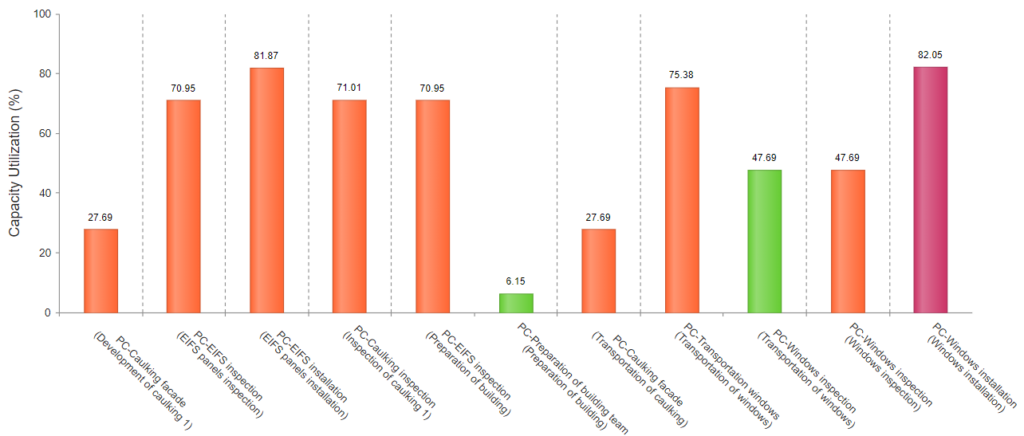
Considering the u of the process centers (PC) is also part of the OS analysis. Figure 6 shows the u of all the PC in the model within their respective product flow. u alongside TH, CT, and WIP, helps the analyst to understand if the production system can afford more WIP, knowing that more WIP would increase the CT. The PC called EIFS installation (PC-EIFS Installation) in the EIFS panels installation product flow shows a u of 81.87%. Since this u is not too close to 100%, it shows that the current WIP can be taken by the production system while avoiding an excessive CT. Figure 6 also shows the bottleneck of the production system. The bottleneck is the resource with the highest u. Here is the PC- Windows Installation in the Windows installation product flow. The resources with a relatively low u can be considered for reassignment. When sharing their capacity with other process centers, they may be able to reach a higher u value and thereby possibly improve in performance relative to this metric. It may also improve system performance especially when it can relieve a resource running too close to capacity.

Discussion

We considered the OS metrics including CT, TH, WIP, u, and the relationships between them as expressed by the VUT equation and Little’s Law to describe the behavior of a production system in construction. In addition, we used the Production Flow graph and the Capacity Utilization graph for the resources included in this production system.

In order to apply OS using the Production Optimizer, we had to make several assumptions some of which highlight some peculiarities of construction production systems:

1. Construction practitioners may lack awareness of the existence of OS metrics or have misconceptions of the implications of amounts of WIP much in excess of what Little’s Law would suggest.
2. Similarly, they may lack understanding of the detrimental impact variability has on system performance, and therefore fail to harness that variability where doing so is possible and affordable. For example, inferior quality causing the need to do rework introduces variability in the system [14]. While we assumed no rework for the system as modeled, the Production Optimizer can account for it. As variability includes process variability or arrival variability caused by product variation (i.e., welding of 2-inch pipe vs. 8-inch pipe), that variation may be needed and desired by the customer.
3. A lack of discipline or ability to stabilize work plans introduces detrimental variability into the system which may result in additional need for inventory, time and capacity.
4. The steady-state assumption may not hold for construction activities that are relatively short in duration. If steady state is not achievable, then DES should be used rather than the Analytical Model. However, the OS framework still applies.

The results of the OS analysis of course need to be viewed in light of the validity of the modeling assumptions made, but this paper showed that an OS model can provide a starting point for PSD of a construction project. An OS model will allow construction professionals to use scientific results to develop their intuition of the production system’s behavior and how their design choices will affect their project’s performance. OS models of the kind presented here are stochastic models and their results are not always self-evident. However, when properly applied, their results will be more realistic than those obtained using deterministic models.

A significant challenge in the application of OS in construction is that production data must be collected on projects—a practice that is not yet so common—to serve as input to the model. To tackle this challenge, we collected data from project team members, then translated this data by making assumptions as needed to be able to go from “project plans” to “production parameters” (i.e., from activity durations to production rates). In addition, we assumed that the SCV value could represent the amount of variability in the system. In construction, it is not common yet to characterize a construction production system by its SCV, therefore, if the SCV is not available, no stochastic model can be developed (whether it is a DES or an analytical model). The quality of this translation and the SCV value are crucial for obtaining reasonable results when creating stochastic models.

Conclusion

This study presented an approach for applying OS to the design of a construction project’s production systems. The literature review and research methods were based on the current use of OS in other industries (the manufacturing industries) to develop our application of OS in construction. The Production Optimizer provided a means to apply an OS analytical modeling to a case study. This case study provided crucial results, which represented the applicability of OS to PSD in construction projects.

It is important to recognize what assumptions had to be made in this SSRRH case study to enable the use of the model and what production data had to be collected from the project team in order to populate the analytical model. Regarding the OS metrics, CT stands out in that it represents changes in WIP and TH, and directly affects project performance (e.g., schedule duration). Finally, the characteristics of the construction process used as a case study (onsite installation, offsite components, building project) can limit the generalization of the results of this study and future research can explore the application of this proposal to other types of construction processes.

Acknowledgments

Special thanks are due to everyone who helped Guillermo Prado Lujan develop his master’s thesis on which this paper is based, namely Iris D. Tommelein, Rhonda Righter, Maria Laura Delle Monache, Roberto J. Arbulu, Patricia Tillmann, Matthew Boersma, Mike Lespron, Anabella Pinon, and Chet Carlson.

References

1. Project Management Institute. A guide of the Project Management Body of Knowledge (PMBOK guide) (6th ed.). Project Management Institute.
2. Shenoy, R., & Zabelle, T. R. (2016). New Era of Project Delivery – Project as Production System. Journal of Project Production Management, 1 (1), 13-24.
3. Ballard, G., Koskela, L., Howell, G., & Zabelle, T. (2001). Production System Design: Work Structuring Revisited. LCI White paper # 11, Lean Construction Institute.
4. Schramm, F K., Rodrigues, A.A. & Formoso, C.T. (2006). The Role of Production System Design in the Management of Complex Projects. Proceedings of the 14th Annual Conference of the International Group of Lean Construction, Santiago, Chile, 227-239.
5. Lee, S., Pena-Mora, F., & Park, M. (2006). Reliability and Stability Buffering Approach: Focusing on the Issues of Errors and Changes in Concurrent Design and Construction Projects. Journal of Construction Engineering and Management, 132(5), 452-464.
6. Russell, M.M., Liu, M., Howell, G., & Hsiang, S.M. (2015). Case Studies of the Allocation and Reduction of Time Buffer through the Use of the Last Planner System. Journal of Construction Engineering and Management, 141(2).
7. Tommelein, I.D. (2020). Takting the Parade of Trades: Use of Capacity Buffers to Gain Workflow Reliability. Proceedings of the 28th Annual Conference of the International Group for Lean Construction, Berkeley, CA, 421-432.
8. Skinner, W. (1985). Manufacturing, The Formidable Competitive Weapon. John Wiley & Sons.
9. Askin, R. G., & Goldberg, J. B. (2002). Design and Analysis of Lean Production Systems. John Wiley.
10. CIRP. (1990). Nomenclature and Definitions for Manufacturing Systems (English Language Version). Annals of the CIRP, 39 (2), CIRP Technical Report, 735-742.
11. Slack, N. Chambers, S., Harland, C., Harrison, A. & Johnston, R. (1998). Operations Management. Atlas.
12. Bellgran, M., & Safsten, K. (2004). Production System Design and Evaluation for Increased System Robustness. Proceedings of the 2nd Second World Conference on POM and 15th Annual18 POM Conference, Cancun, Mexico.
13. Koskela, L. (1992). Application of the New Production Philosophy to Construction. Technical Report No. 72, CIFE, Stanford University, Stanford, CA.
14. Tommelein, I.D. (1998). Pull-Driven Scheduling for Pipe-Spool Installation: Simulation of a Lean Construction Technique.” Journal of Construction Engineering and Management, 124(4) 279-288, doi.org/10.1061/(ASCE)0733-9364(1998)124:4(279)
15. Martinez, J. C. (1996). STROBOSCOPE State and Resource Based Simulation of Construction Processes. Ph.D. Dissertation, Civil & Environmental Engineering Program, University of Michigan, Ann Arbor, MI.
16. Tommelein, I. D. (2006). Process Benefits from Use of Standard Products – Simulation Experiments Using the Pipe Spool Model. Proceedings of the 14th Annual Conference of the International Group for Lean Construction, Santiago, Chile, 177-188.
17. Ballard, G., & Howell, G. (1998). What kind of production is construction? Proceedings of the 6th Annual Conference of the International Group for Lean Construction, Guaruja, Brazil.
18. Koskela, L., & Ballard, G. (2003). What Should We Require from a Production System in Construction? Construction Research Congress, ASCE, Honolulu, Hawaii, 1-8.
19. Schramm, F. K., Costa, D. B., & Formoso, C. T. (2004). The Design of Production System in Low- Income Housing Projects. Proceedings of the 12th Annual Conference of the International Group for Lean Construction, Helsingør, Denmark.
20. Kemmer, S. L., Heineck, L. F. M. & Alves, T. C. (2008). Using the Line of Balance for Production System Design. Proceedings of the 16th Annual Conference of the International Group for Lean Construction, Manchester, UK, 299-308.
21. Schramm, F. K., Tillmann, P. A., Berr, L. R., & Formoso, C. T. (2009). Redesigning the Production System to Increase Flexibility in House Building Projects. Proceedings of the 17th Annual Conference of the International Group for Lean Construction, Taipei, Taiwan, 347-358.
22. Murguia, D., & Urbina, A. (2018). Complex Production Systems: Non-Linear and Non-Repetitive Projects. Proceedings of the 26th Annual Conference of the International Group for Lean Construction, Chennai, India, 858-868.
23. Barth, K.B., Sterzi, M.S., Formoso, C.T, Alliende, J.I, Bertín, D., & Del Rio, J. (2020). Implementation of Production System Design in House Building Projects: A Lean Journey in Chile. Proceedings of the 28th Annual Conference of the International Group for Lean Construction, Berkeley, CA, 397-408.
24. Hopp, W. J., & M.L. Spearman. (2008). Factory Physics (3rd ed.). Waveland Press, Inc.
25. Pound, E., Bell, J., & Spearman, M. (2014). Factory Physics for Managers. McGraw-Hill.
26. Krajewski, L. J., & Ritzman, L. P. (2001). Operations Management: Strategy and Analysis (6th ed.). Prentice Hall.
27. Adam, E. E. (1983). Towards a Typology of Production and Operations Management Systems Academy of Management Review, 8 (3), 365-375.
28. 32.Swamidass, P. M. (1991). Empirical Science: New Frontier in Operations Management Research. Academy of Management Review, 16 (4), 793-814.
29. Zandin, K. B. (2001). Maynard’s Industrial Engineering Handbook (5th ed). McGraw-Hill.
30. Ackoff, R. L. (1956). The development of Operations Research as a Science. The Journal of the Operations Research Society of America. 4 (3), 265-295.
31. Heiman, D. W. (1960). Operations Research as Applied to Construction. Management Technology, 1(2), 20-25.
32. Fuller, J. A. (2005). Operations Research and Operations Management: From Selective Optimization to System Optimization. Journal of Business & Economics Research, 3(7), 11-16.
33. Chase, R., Aquilano, N., & Jacobs, R. (2001). Operations Management for Competitive Advantage (9th ed.). McGraw-Hill.
34. Factory Physics. (2022). Operations Science. https://factoryphysics.com/operations-science (accessed September 2022).
35. Project Production Institute. (2022). Glossary. https://projectproduction.org/resources/glossary/ (accessed September 2022).
36. Spearman, W., & Spearman, M. (2020). Data Science vs Operations Science. Presentation at the 2020 7th Annual PPI Symposium. Event held virtually.
37. Shenoy, R. (2017). A Comparison of Lean Construction with Project Production Management. Journal of Project Production Management. 2 (1), 35-47.
38. Prado, G. (2022). Operations Management Concepts Applied to Offsite Construction. Proceedings of 2022 Modular and Offsite Construction (MOC) Summit, Edmonton, Canada, 225-232.
39. Ballard, G., & Arbulu, R. (2004). Making Prefabrication Lean. Proceedings of the 12th Annual Conference of the International Group for Lean Construction. Helsingør, Denmark.
40. Project Production Systems Laboratory. (2022). Glossary. https://p2sl.berkeley.edu/glossary/ knowledge-center-glossaryatoz/ (accessed October 2022).
41. Roser, C. (2017). The Kingman Formula – Variation, Utilization, and Lead Time. https://www.allaboutlean.com/kingman-formula/ (accessed October 2022).
42. Gharaie, E., Blismas, N. & Wakefield, R. (2012). Little’s Law for the U.S House Building Industry. Proceedings of the 20th Annual Conference of the International Group for Lean Construction, San Diego, CA.
43. Sutter Health. (2022). The New Sutter Santa Rosa Building. https://www.sutterhealth.org/about/building-ssrrh (accessed November 2022).
44. The Boldt Company. (2022). Sutter Health - Santa Rosa Regional Hospital https://www.boldt.com/project/sutter-health-santa-rosa-regional-hospital/ (accessed December 2022).
45. Herrero Builders. (2022). Sutter Santa Rosa Regional Hospital Expansion Project. https://www.herrero.com/projects/sutter-santa-rosa-regional-hospital-expansion#:~:text=The%20expansion%20adds%2058%2C000%20square,post%2Danesthesia%20care%20unit%20bays (accessed November 2022).
46. Prado, G. (2022). Impact of Production Systems Design on Project Performance: An Operations Science Analysis on a Case Study in Construction. Master of Science Thesis, Engineering and Project Management Program, University of California, Berkeley, CA.
47. Georgy, S. (2019). PPI Process Mapper. Journal of Project Production Management, 4 (1), 104-111