This paper investigates how variability in the scope of construction work packages—particularly size-based differences in arrival and service times—affects project performance metrics like completion time, work-in-process (WIP), and cycle time (CT). Using discrete event simulation (DES), the study compares traditional M/M/1 queue behavior with more realistic production systems exhibiting scope-induced correlations with the goal of delivering analytical heuristics for DES results. Due to the transitory nature of construction projects, discrete event simulation is more appropriate than analytical methods. The findings reveal that even with equal average arrival and service rates, variability in scope introduces nonlinear effects on project duration and throughput due to correlations and sequencing. Managerial strategies like scope normalization, sequencing, and buffered releases are recommended to mitigate these impacts and reduce rework risks.

Bio coming soon

Ivan D. Damnjanovic is Professor and the Director of Engineering Project Management program at Texas A&M University. Dr. Damnjanovic specializes in qualitative and quantitative methods for management of engineering and project risks as well as management of infrastructure and transportation systems. He has an extensive experience in engineering r ...
One of the most important sources of variability in project production is the variability in scope of work packages that flow through the production systems. This work package variability originates from the way project scope of work is developed and sequenced. For example, a work sequence for installation of pipe spools may include different size spools flowing through the production system. As a result, production process exhibits variability.
The scope variability has some unique features. It is not the same as regular variability due to randomness in arrival and server processing times/rates for the same scope work, but it is an added variability that affects both the arrival and service rates. For example, consider two types of work packages (big and small). The overall system variability then depends not only on the consistency in time to complete each individual work package (big or small), but also on the variability due differences in the time to complete “large” versus “small” work packages.
Statistically, the scope variability is manifested as a correlation between the arrival rate of work packages and the service rate. For example, bigger work packages are processed longer and hence flow slower through the production system, and conversely, smaller packages are processed shorter and flow faster. Hence, the arrival and service rates are highly correlated, which violates the Markovian assumption in M/M/1 queues. Kingman's formula also known as VUT equation provides some insights in the effect of variability in server and arrival rate, utilization on expected cycle time on generalized queues. Still, it does not consider correlation between the arrival and service rates.
The G/G/1 type queues are considered a more generalized description of project production systems. However, due to their complexity, closed-form solutions are typically not available. Hence, to gain insights in how production systems perform one needs to run discrete event simulations. While informative, simulations are subjected to assumptions and modeling decisions, and not good at providing the sensitivity between the key variables. Hence, heuristics are often developed to show the simplified relationship between the key variables.
One way to look at the work package variability and the resulting correlations is to consider system operating regimes. For example, our production system can operate in regime “Slow” where the arrival rate is slow and the processing times are slow, or regime ‘Fast” where arrival rate is fast and the processing times are fast. This is sometimes referred to as a modulated process. More specifically, it is referred to as Markov Modulated Quasi Birth Dead Process (MMQBDP) where modulation enables Markovian behavior. However, closed-form solutions are easily derived only for simplified cases such as Markov Arrival Process (MAP).
The objective of this paper is to develop project management insights of the impact of scope variability on project completion time, contingency, and other metrics of production systems such as cycle time and WIP. We analyze the impact of work package variability on project completion time and contingency as well on other important production performance metrics that can be considered leading indicators of rework risk. We consider two different situations, one where the arrival times are determined by random switching between two arrival streams with different rates, and one where we adjust the rates to maintain the average interarrival times.
Discrete Event Simulation (DES) has been widely adopted in the construction domain to model, analyze, and optimize production processes that are inherently stochastic and resource-constrained. In construction, DES is particularly effective because it can capture the transient and project-specific nature of operations, including task sequencing, resource availability, and environmental variability [1, 2, 5]. Prior studies have applied DES to a wide range of construction problems such as earthmoving operations, concrete delivery scheduling, and modular assembly, demonstrating that DES can outperform analytical methods when process variability is high and system configurations are complex [3, 4]. Unlike steady-state manufacturing systems, construction projects are multi-variable, dynamic systems where the production environment and job characteristics evolve over time, making DES an ideal choice for capturing both short-term fluctuations and long-term performance trends.
A specific challenge in construction process modeling is the correlation between arrival and service rates, which often arises from variability in the scope or complexity of work packages. When larger, more complex tasks take longer to process and simultaneously arrive at a slower rate, the arrival and service processes become statistically dependent—a condition that violates the assumptions of traditional M/M/1 queue models [6, 8, 14]. Kingman’s VUT equation provides an analytical link between variability, utilization, and cycle time for generalized queues [7], but it does not account for this correlation. As a result, systems exhibiting such dependencies can show significantly different performance patterns compared to independent-arrival systems, particularly under conditions of high utilization. This has led to interest in modeling frameworks that can explicitly handle correlated variability and non-Markovian dynamics [12, 13].
In queueing theory, modulated processes provide a way to represent systems whose parameters shift between distinct states. The Markov-Modulated Poisson Process (MMPP) extends the classical Poisson process by allowing the arrival rate to vary according to an external stochastic mechanism, often a Markov chain [9, 10]. When both arrival and service rates are subject to such modulation, the system can be modeled as a Markov-Modulated Birth–Death Process (MMBDP), or in more complex forms, as a Markov-Modulated Quasi-Birth–Death Process (MMQBDP) [11]. While closed-form analytical solutions exist for special cases like the Markov Arrival Process (MAP), most realistic configurations—especially those with multiple correlated job classes—require simulation-based approaches to estimate performance metrics. Applications of these models in construction have been limited, but in related fields like telecommunications and manufacturing, they have been used to study bursty arrivals, correlated workloads, and service interruptions [9, 10].
This research builds on the foundation of applying DES to examine the effects of scope-induced correlation between arrival and service rates in construction project production systems. We evaluate multiple operating systems—from independent Poisson arrivals to fully correlated modulated processes—and quantify their impacts on project completion time, work-in-process, and cycle time under different levels of variability and utilization. The goal is to develop practical insights and heuristics for construction managers, showing that even with identical average rates, correlated or sequenced variability can introduce nonlinear delays and congestion effects. This work addresses a gap in the literature by explicitly modeling and quantifying the combined effects of correlation, scope variability, and process modulation in construction systems, thereby informing strategies for risk mitigation and performance optimization.
The remaining of this paper is organized as follows. First, we introduce the cases that correspond to different approximations of production systems under work package scope variability. The objectives of this contrasts M/M/1 results to more realistic cases of production systems. Second, we present the comparison results, followed by the discussion on key findings. Finally, we present summary and the direction for future research.
As previously mentioned, we contrast the baseline M/M/1 case (Case A) against multiple other cases with more assumptions of production system with work package scope variability (Cases B-D). Finally, we also consider a special case (Case E) where different scope packages are processed sequentially – first all large and then all small.
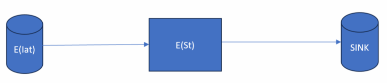
Case A depicts an original M/M/1 queuing system where the arrivals follow a Poisson process, meaning the interarrival times are exponentially distributed with a rate of λ. The service times are also exponentially distributed with rate μ. Only one server handles all the jobs that arrive. This type of system is often used as a simplification of the real situation. The completion time to “n-th” arrivals to the sink is an Erlang distribution. In this case 1,000 work packages are processed through the system. Due to the central limit theorem, the time to the 1,000th arrival can also be approximated by a normal distribution. The sum of a large number of independent and identically distributed random variables with finite mean and variance tends toward a normal distribution, regardless of the original distribution. Figure 1 shows the Case A setup.
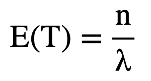
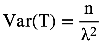
Analytically, the expectation and the variance of duration or project time can be found using the following formulas where n represents the number of work packages in the system and λ is the mean arrival rate.
(1)
(2)
(3)
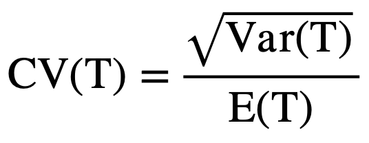
For example, with the 1,000 work package scenario, the coefficient of variation (CV) of the completion time is equal to:
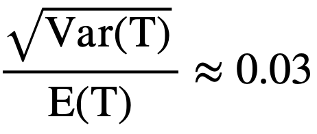
Based on analytical methods, this states the standard deviation of the completion time is only 3% of the overall mean. Construction projects typically have much larger variation than 3%, which can provide a false sense of security when checking completion time and not accurately accounting for the correlation between arrival rates and service rates.
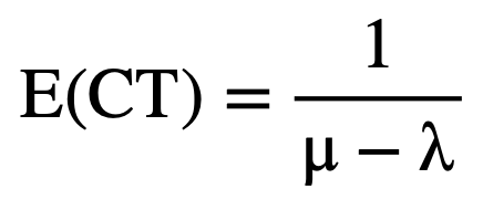
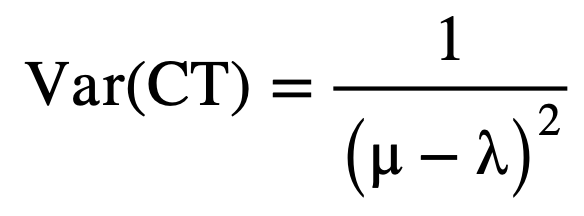
Analytically, the total cycle time, E(CT) – defined as the time a job spends in the system from its arrival to its departure – is the sum of waiting and service time. While the two components are stochastic on their own, the memoryless nature of the exponential arrival and service times result in a system where the distribution of the total cycle time also follows an exponential distribution, but with a new rate parameter that equals (μ-λ). For a steady-state and stable system, the expectation and the variance of cycle time can be defined analytically by the following equations:
(4)
(5)
For M/M/1 queues, Work- In- Process, or the number of jobs in a system at any given time, follows a geometric distribution. Because arrivals and service completions occur randomly, the WIP levels naturally fluctuate over time.
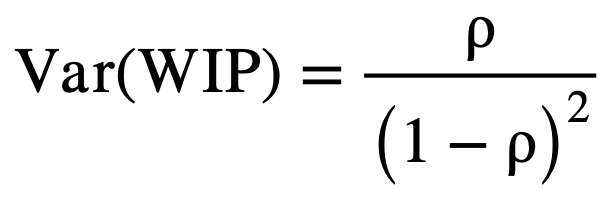
Analytically, WIP directly depends only on utilization:
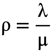
As utilization of the server increases, the system becomes more congested leading to longer delays and greater accumulation of work packages in the system. In extreme cases, as ρ approaches 1, the system approaches instability, where WIP and delays grow without bound. The expected number of jobs in the system and its variance are given by:
(6)
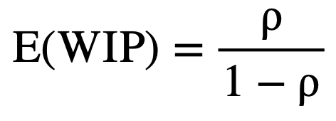
(7)
Again, Case A serves as the baseline for our analysis, as it reflects a fundamental model in queueing theory. Its simplicity and analytical clarity make it an ideal reference for evaluating more complex systems.
To better represent a more realistic construction system, Case B models a general MMQBDP (Markovian Multi-class Queue with Birth-Death Process) framework. This case captures two distinct and correlated job classes—fast and slow—with differing arrival and service characteristics. For simplicity, each job type arrives independently with equal probability (50%). However, their arrival and service times are inter-dependent, meaning fast arrivals tend to have faster service times and slow arrivals tend to require longer service. This setup more accurately reflects midstream dynamics commonly observed in real-world construction workflows, where job complexity and service demand are not uniform across all arrivals. Figure 2 shows the system structure for Case B.
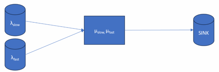
Note that we do not have a closed-form solution for expectation and variance. These values will be estimated using discrete event simulation and compared to baseline Case A.
Case C models a system in which arrivals are consistent and estimated with a mean interarrival rate. In other words, the work packages arrive independently of their size. This can be reflective of an initial activity/task where the work packages are released without consideration of their size (upstream). Alternatively, this can reflect a situation where arrival rates are stabilized midstream and passed to remaining activities/tasks at the constant rates.
Hence, unlike previous cases, the variability in the system is concentrated in the server, which handles two distinct service times: one for fast work packages and one for slow work packages. This configuration results in minimal variability in arrival times, while the service process exhibits high variability due to the presence of two different job types. Such a setup is useful for analyzing how processing-time alone can impact system performance, independent of arrival randomness. Figure 3 shows the setup for Case C.
Again, note that we do not have a closed-form solution for expectation and variance. These values will be estimated using discrete event simulation and compared to baseline Case A.
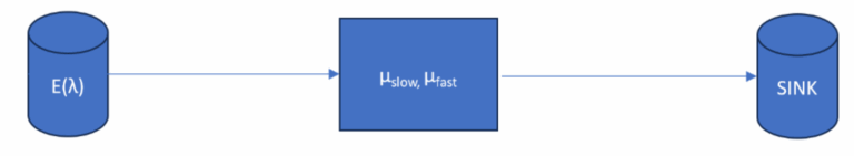
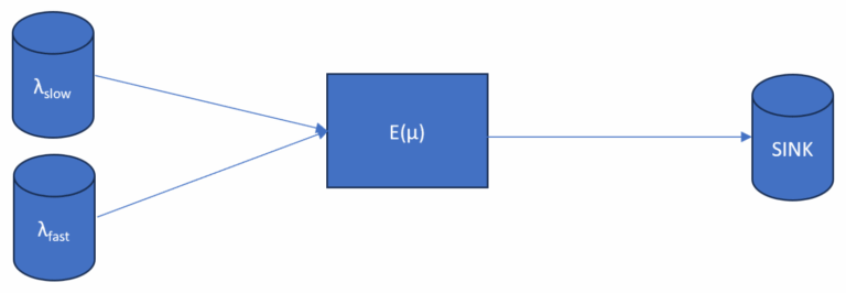
Case D serves as a benchmark scenario designed to isolate the effects of arrival variability that is not correlated with service time variability. In this model, arrivals are drawn from a mixture of exponential interarrival times—representing both fast and slow streams—creating a modulated Poisson process. However, all jobs are processed with the same average service time, removing variability from the service process itself. This configuration allows focused analysis on how fluctuations in arrival patterns alone impact the system.
Case D can also be reflective of a situation downstream production process where the scope of work packages does not impact the service time of the activity. For example, testing or administrative processing of completed work packages may not depend on the size of the work package. Figure 4 shows the system setup for Case D.
Even though Case D can be analytically traced and represented as modulated Poisson process, we still use discrete event simulation (DES) to estimate expectation and variance of the key production metrics.
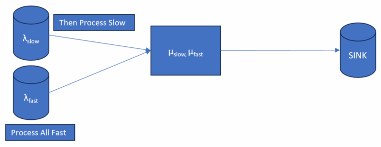
Case E introduces a management strategy to sequence processing of work packages, where all of the fast jobs are processed first, followed then by the slow jobs, each with their own corresponding service time. This setup models a two-phase system where the parameters of Cycle Time, WIP, and Throughput depend on which work package is currently in service. Both, the arrival and service processes are structured as a sum of two different Erlang distributions, each representing the slow and fast work package classes with distinct scale parameters. Rather than mixing the work packages, this case explores the effect of ordered heterogeneity in terms of arrival and service times. As the Erlang shape parameter grows large, the arrival and service times approach a normal distribution under the central limit theorem as seen before. Thus, when summing the two distinct Erlangs (fast and slow), the total processing time also begins to approximate a normal distribution, though not symmetric due to the differing scale parameters. This case allows the use of analytical methods to approximate how the system will react. Figure 5 shows the system setup for Case E.
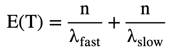
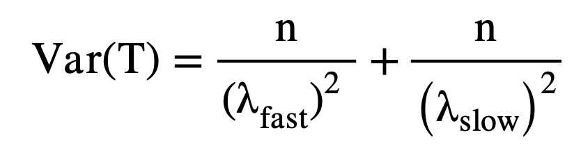
The total project time can be found by using the sum of two erlang distributions. Again, if n, or number of work packages, is large, the distributions will approach normal.
(8)
(9)
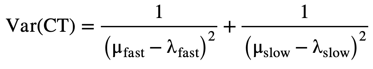
Cycle Time can be defined as a hypoexponential, which defines the sum of n independent but non-identically distributed exponential random variables.
(10)
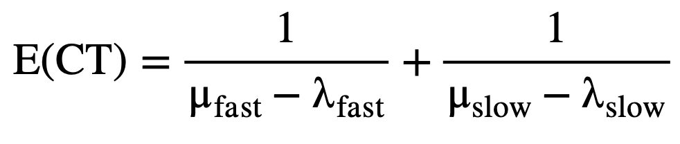
(11)
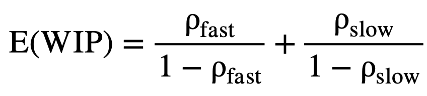
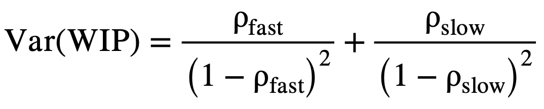
Since WIP is being modeled as a sum of geometric stages, each with a success rate p = 1-ρ, it becomes a negative binomial in the case of the same utilization rate, ρ. The Negative Binomial distribution gives the probability of observing n failures before r successes. In this framework, the total number of work packages still in the system behaves like the number of failures before r successes.
(12)
(13)
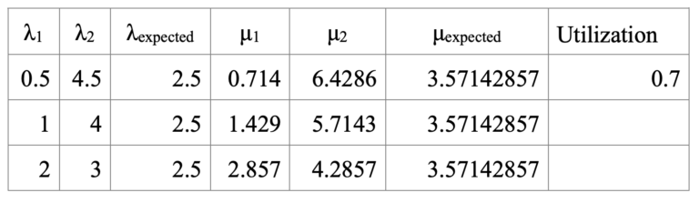
To begin, a utilization, or ρ, of 50% was used to determine a baseline result for Cases A – E. The values used are found in Table 1 below.
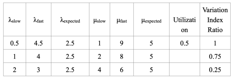
In the following figures depicting the results, the x-axis represents the Variation Index Ratio (VIR), a normalized measure of how different the fast and slow arrival/service rates are, expressed as a fraction of the largest variation observed in the dataset which is also seen in Table 1.
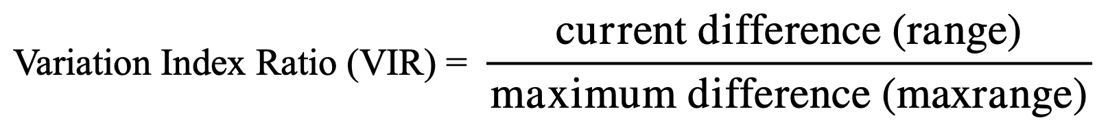
The VIR is calculated to compare the effect of different amounts of variance while keeping the same mean value. For each arrival and service rate pair (λfast,λslow) and (μfast,μslow), the absolute difference is computed:
(14)

The maximum of these differences across all cases is identified as the reference range. For each case, the current difference is divided by this reference range to yield the VIR:
(15)
In other words, this metric shows the effect of variation in the system metrics. For example, based on the arrival rates in Table 1, λfast is equal to 4.5 minus λslow which is equal to 0.5 which becomes a max range and current range of 4 since it is the point of largest variation. Therefore, the VIR is equal to 1 (4 / 4). For the second case of variation, λfast is equal to 4 minus λslow which is equal to 1 creating a range of 3. This is not larger than the maximum range found above, therefore the VIR will be 3 divided by 4, equaling 0.75. Lastly, the smallest case of variation λfast is equal to 3 minus λslow which is equal to 2 creating a range of 1. The VIR is found to be 0.25.
The values used for arrival rate and service rate have mean values of 2.5 and 5 work packages per day respectively. The difference is in the range between the values. For example, the first set of arrival rates has the highest range ( 4.5 – 0.5 = 4), but still has a mean arrival rate of 2.5. While the last set of arrival rates has the lowest range (3 – 2 =1), and still has the mean arrival rate of 2.5. The same process was used for the service rates as well. For Case A and E, the analytical formulas were used to find the results of Project Completion Time, Work In Process, Cycle Time, and Interdeparture Time. For Cases B – D the results were found using discrete event simulation.
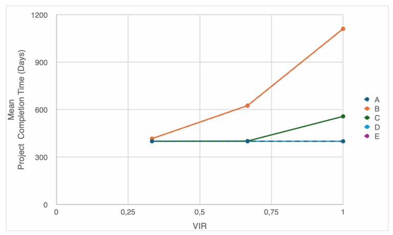
The results of the analysis are shown in Figures 6–14. With little/ no variation between arrival rates, the project completion time stays steady for all five cases around 400 days. Although, when variance is introduced the completion time for Case B and E changes drastically, more than doubling even though the arrival and service rates have the same mean values. This is a result of Jensen’s inequality.
Case D shows no change in project completion time even with a change of variance in arrival rates, which is expected as the inter-departure rate depend only on the average arrival rate. While Case C sees an uptick in duration as the variance is shown in the most extreme case of arrival variability, which is the result of a case where arrival rate is greater than service rate. Figure 6 summarizes the results.
From the perspective of variance, which is critical if we are to set contingency, we see similar trends (see Figure 7).
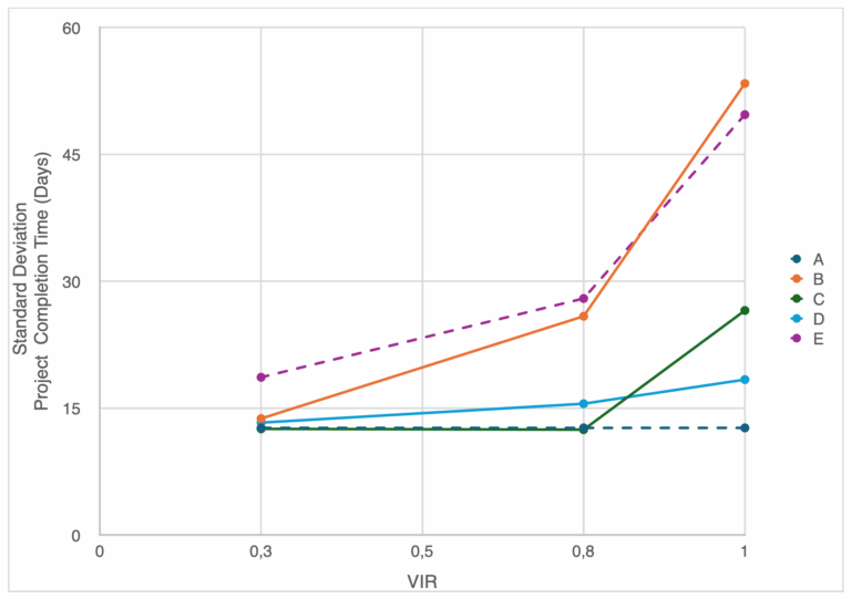
The system structure, being the configuration and logical organization of how work packages are processed (i.e. Cases A – E), and correlation between work package types, not just the arrival and service variance drive variability in project duration outcomes. Case A offers consistency under all variance conditions, while systems with correlated or sequenced workloads like B and E experience high fluctuations in project completion time even at the same utilization levels. This is important in construction due to the criticality of reliability and schedule predictability which can be just as important as the average performance.
However, it is important to note that the variability for all cases is relatively small when compared to the mean value. This is the result of the nature of aggregating variability in completion of N-th items.
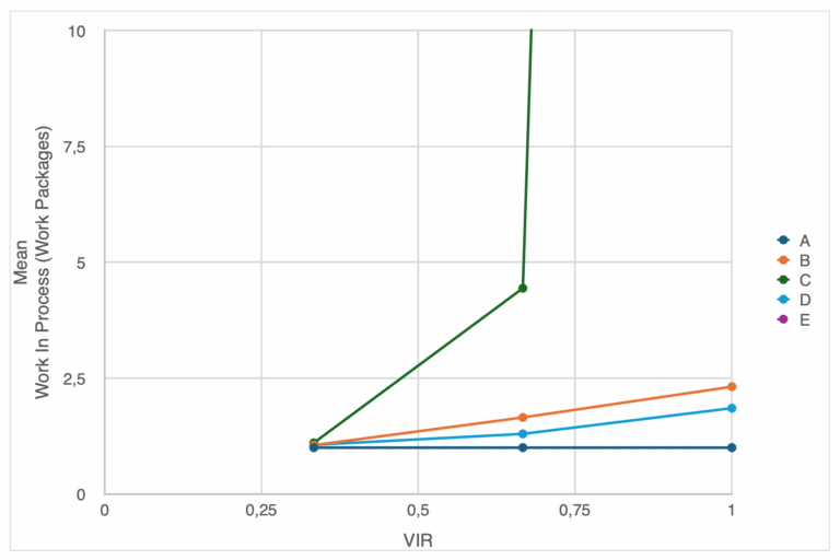
In terms of Work in Process, the variability in arrivals and service rates both have a more significant impact on the performance. For Case A, WIP remains low and stable across all levels of variance, as expected from the memoryless, exponentially distributed system. Case B has correlated variability in arrival and service rates, which causes WIP to increase moderately with the variance. Correlation between the slow and fast arrivals and service cause clustering which leads to short bursts of congestion in the queue, driving up the WIP. Case C has stable arrivals, but variability in service rates which causes WIP to spike dramatically as the variance becomes higher. This shows how variability in the server alone can highly impact WIP, even under steady state arrivals. Large service times cause the queue to build up quickly, causing the system to push an unsteady state. With only introducing variability in the arrivals, as done in Case D, WIP stays rather close to A, validating that arrival variability is not the sole driver in a drastic increase system congestion when service time remains constant. Due to Case E being the sum of two Erlang Distributions, WIP is kept constant. The results are summarized in Figure 8.
Cycle time follows a similar pattern as WIP, with slight changes. For Case A and D, cycle time remains flat, predictable, and consistent. Constant service rates keep delays minimal and stable within the system. Case B shows moderate growth in cycle time with variance, due to the same correlation-induced queuing as seen in WIP. Case C shows a sharp increase in Cycle Time, mirroring the WIP spike. With variability in service rates and routine arrivals, the system suffers from significant delays when the slower jobs are blocking the server. Case E shows gradual growth in cycle time, due to the effect of deterministic sequencing. Even if the arrivals are orderly, larger jobs delay the system’s throughput pace.
To get a better idea of how the systems preform under different loads, the arrival rates were adjusted for levels of 30% and 70% utilization (see Table 2 and 3 below).

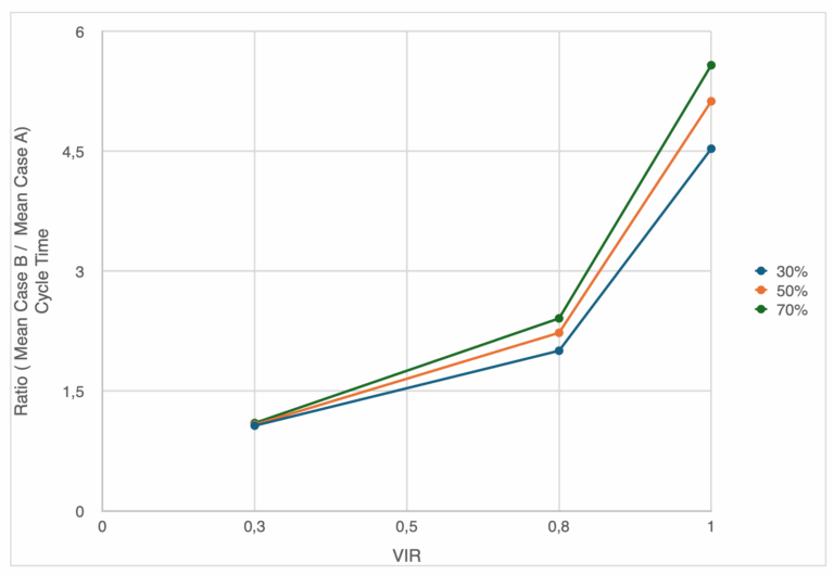
The ratios are computed using Case A as a baseline. The y-axis shows the ratio of project duration:
(16)
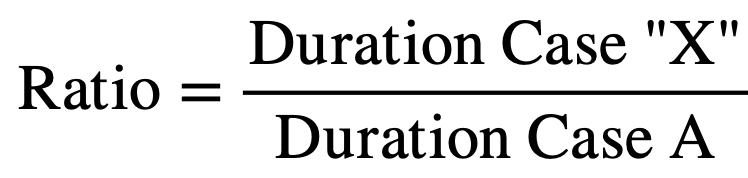
Figure 9 shows the effect of the ratio. The values greater than 1 indicate that Case “X” performs worse than Case A, and values near 1 indicate similar performance as the baseline case. This is for the same type of work package scope variance. The x-axis shows increasing variance in the arrival or service process as before.
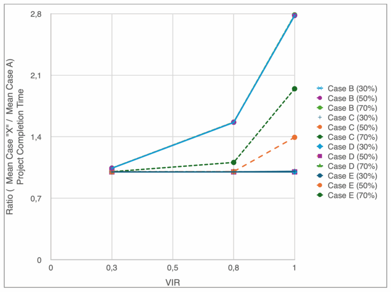
For Case B, the impact of variance is minimal at 30% and 50% utilization, but explodes at 70% utilization. This shows that correlated job classes become problematic only as the system nears full utilization, where bursts of slow work packages align with limited service availability that compounds the delays. With Case C we see the project duration grow more steadily across utilization levels, especially as the variance becomes higher. This supports the results seen earlier; server variability is enough to degrade the system performance even if the arrivals are steady, and especially under heavier loads. Case D is interesting in that even with the variation in arrivals, the ratio remains around 1 for all utilization levels and variance. Unstructured arrival variability is not always harmful when service times are stable. Although, Case E shows a degradation in performance substantially at 70% utilization. This reflects the effect of sequencing jobs can have on a project, leading to delays that ripple throughout the project that amplifies risk.
Case B vs Case A Ratio: In general, there is no impact on utilization on the ratio for completion time and inter-departure times. Only scope variability is increasing the ratio. This does not mean that utilization is not affecting completion time; it does. What it means is that completion time for Case A and B equally increases with increased utilization. However, this is not the case for CT and WIP. The impact of scope variability on CT and WIP for Case B is higher relative to Case A at higher utilization level. For example. Expected CT for higher level of scope variability increases to almost five times the levels seen for Case A (see Figure 10).
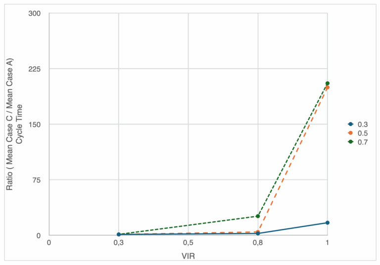
Case C vs Case A Ratio: As previously mentioned, completion time and inter-departure times are affected with an increased in both scope variance and utilization level. This again because we have a higher chance of a situation where utilization is higher than one, and therefore inter-departure times becomes governed by the service rate, not arrival rate. The expected duration can almost double with increased variance.
Case C is where scope variability creates the highest impact on CT and WIP. In fact, the extreme scope variances can increase WIP/CT levels to extreme values. This is because the gap between the service rate and the arrival rate because large, and as a result creates long queues and waiting times (see Figure 11).
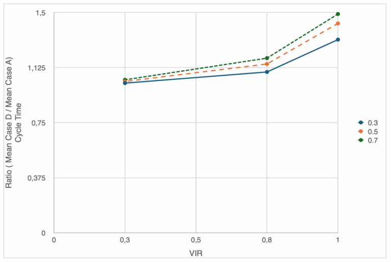
Case D vs Case A Ratio: In general, and similar to Case B to Case A ratios, there is no impact on utilization on the ratio for completion time and inter-departure times. Only scope variability impacts them. It is the same situation for CT and WIP as or Case B/A ratios. However, the impact is smaller. For example, where the impact of Case B relative to Case A was in order of five, for the ratio of Case D to Case B is only 50 percent. This is because service time in Case B is not affected by scope variability (see Figure 12).
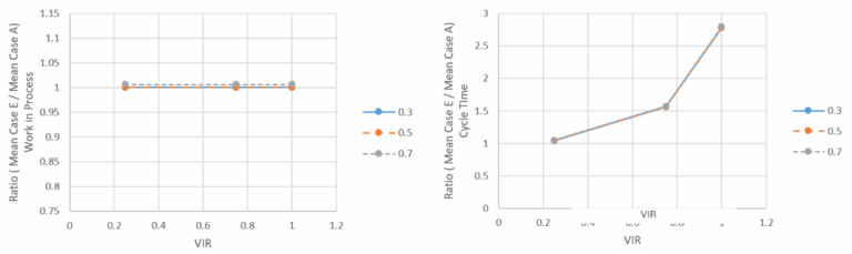
Case E vs Case A Ratio: Both completion time and inter-departure times ratios to Case A are impacted by utilization. However, it is important to note that it is still impacted by scope variability. Basically, Case E performs similar to Case B from the perspective of completion time. However, from WIP viewpoint, Case E acts exactly as Case A. Hence it is not impacted by scope variability. It is impacted by utilization, but at the same levels as Case A. CT is impacted but only the scope variability, not with increase in utilization (see Figure 14).
Introducing different arrival rates for different scope work package not only increase the variance in total completion requiring higher contingency, but also effectively slows down the production, decreasing the throughput i.e. increasing the mean completion times. This is because upstream crews are switching between two different regimes of processing - small and large work packages.
Why is this the case? A simple answer is that E(1/λ) is not equal to 1/E(λ). As previously mentioned, based on Jensen’s inequality, the average of convex function will always be greater (or equal to) than the function of the averages. Practically, switching between the slow and fast streams with equal probability creates arrival times that are skewed towards the slower process. For example, if we want to maintain the average interarrival times of 0.4 based on the average arrival rate of 2.5, and where slow packages arrive at rate of 1 and fast arrive at the rate of 4, we need to adjust the probability of switching from 50 percent to 80 percent to get the same interarrival times of 0.4.
The Coefficient of Variation (CV) in project completion time is relatively small, hence, the impact of increased variability on the contingency is not significant.
We have that:

, where n is number of work packages to be completed. As previously mentioned, this is due to “averaging the averages” and the nature of Erlang distribution that characterizes the time to n-th work package completion. For a large number of work packages, due to the Central Limit Theorem, completion time distribution can be considered Gauss-Normal which further simplifies estimating the contingencies based on required percentiles.
Increased levels of WIP and CT in the system can be considered a leading indicator of rework risk. The risk impact is determined by the size the WIP and duration of CT if the items need to be reworked. The results show that WIP and CT in general increase with increased scope variability and utilization. The results are more significant for Case C where the arrival rate is considered an average and not matched with service rate.
Consider making less variable in scope; again, if it makes sense from the viewpoint of how you develop the work packages.
Process small and then large work packages, or vice versa. This breaks down variability and allows for reducing WIP and CT. Project duration still remains sensitive to scope variability. This approach sometime might work, but again it depends on the sequencing of installation; also consider mixing different scopes at the beginning to check for the rework risk, and only then processing them separately.
Introduce a buffer to eliminate added upstream variability; note that this is not a good idea if the next activities/tasks are also affected by the same scope variability. It this is case, avoid releasing work packages at different sizes at the same rate. The impact of this is significant on completion time, and highly severe on CT and WIP.
Consider adjusting the arrival rates to match average inter-arrival times to start with. This approach helps with completion time. It will remain constant even if we increase variability in scope of work packages.
This study explores how variability in the scope of construction work packages—particularly differences in size that influence both arrival and service times—affects key project performance indicators such as completion time, work-in-process (WIP), and cycle time (CT). By modeling five queueing scenarios, including the classic M/M/1 system and more realistic cases with correlated or sequenced variability, the paper highlights how even systems with identical average rates can perform very differently under varying scopes. Simulations reveal that correlated or sequenced processing (Cases B and E) and variability in service times (Case C) significantly degrade system performance, especially under high utilization. In contrast, variability in arrival times alone (Case D) has a smaller effect if service rates remain constant.
The findings underscore that scope-induced variability introduces nonlinear and often hidden risks to project timelines and system stability. Managers are advised to minimize variability in work package scope where feasible, sequence tasks strategically, and align arrival rates with expected service capacity. Importantly, while average performance may appear acceptable, increased variance can substantially increase delays and rework risks—especially under higher utilization. Understanding and planning for these dynamics is essential to improve reliability and optimize production in complex construction environments.