
Deep excavation sites produce large volumes of visual records without panel-level temporal traceability: a photograph alone cannot indicate when a specific wall panel entered a given phase, how long it remained there, or what production state corresponded to that moment. This paper presents a preliminary Project Production Management (PPM) framework based on computer vision to transform UAV observations into auditable production events in anchored shotcrete retaining walls. The system combines an EfficientNet-B0 classifier that identifies the construction phase of a wall panel, a YOLOv11 detector that localizes and counts five crew categories, and a temporal inference layer that assigns PPM states through phase-crew-sequence correspondence rules. The classification layer was validated on 13,706 real field images; the optimized EfficientNet-B0 achieved 97.15% accuracy and a macro F1-score of 0.9685 under real-site conditions. Crew detection and PPM inference are demonstrated through a proof of concept on a representative steel-phase UAV sequence, generating a balance chart, temporal crew counts, visual labor-time, and a process map. The central finding is that the same visual phase can contain distinct production states, productive installation, waiting, transition/support, and inspection/release, confirming that phase and crew integration produces flow data that image classification alone cannot yield.
Keywords: Project Production Management; Operations Science; computer vision; CNN; anchored shotcrete retaining walls; WIP; throughput; cycle time; crew analysis; UAV; YOLOv11; EfficientNet-B0.

William Yalico is a final-year Civil Engineering student at the University of Engineering and Technology (UTEC), Peru, and a Project Control Intern at COSAPI S.A., a leading construction company with over 65 years of experience in Peru. He is a recipient of the Beca 18 scholarship, awarded by the Peruvian government for academic excellence, and has p ...
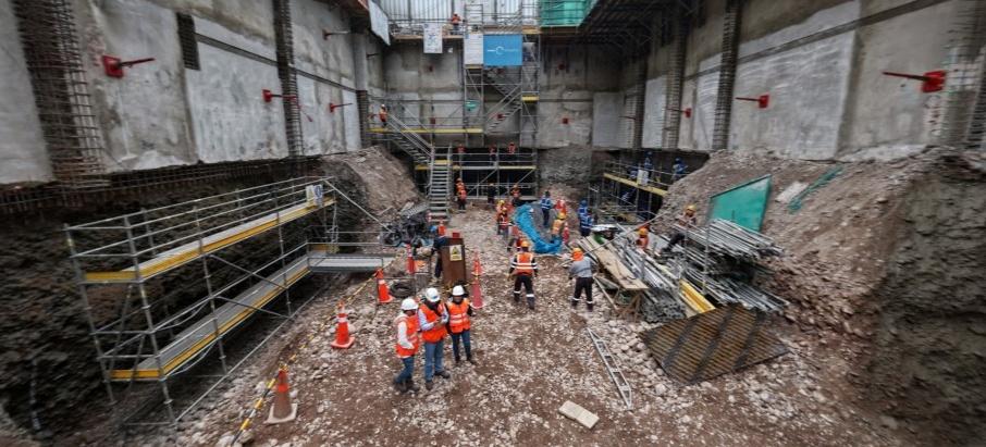
Complex construction projects require production-system observability to control flow, resources, and constraints. From a PPM perspective, a project is a temporary production system in which materials, information, crews, and work packages move through interdependent operations [1]. In Operations Science, production performance is governed by work-in-process (WIP), throughput, cycle time, and variability [2]. Improving control therefore requires first converting field execution into observable production data. In anchored shotcrete retaining walls, each wall panel progresses through a sequential process: profiling, steel reinforcement, shotcrete, and perforation/anchoring. In practice, this sequence is executed with simultaneous fronts, mobile crews, scaffolds, inspections, cleaning, manual filling, waiting between stations, and dependencies on specialized equipment. The problem is therefore not only to recognize a construction phase in an image, but to identify the production state of a panel within a flow sequence. Integrated project delivery and digital coordination have underscored the need for reliable production information across project teams [3]. Computer vision has demonstrated potential for construction progress monitoring, object detection, workforce activity analysis, and safety monitoring [4]-[6], [11]. A recent paper at the PPI 3rd Annual Technical Conference applied YOLOv8 to automatically extract operation start and end times for slab concrete pouring from site video [13]. The present work extends that approach by classifying four construction phases in a more complex sequential process, detecting five crew categories, and inferring five PPM states, including waiting and candidate constraint, in the context of anchored shotcrete retaining walls. This paper introduces an intermediate layer between visual perception and production control in which model outputs are translated into interpretable production events. The analyzed construction context involves multiple simultaneous work fronts, panels in different states, and mobile resources, as shown in Fig. 1.
The preliminary framework is organized around four operational questions: what does the system see, who does it see, what are they doing, and how are they doing it? The first two correspond to visual perception; the last two correspond to production-state inference and visual flow metrics.
Construction sites generate photographs, videos, daily reports, crew records, lookahead plans, and progress logs. These inputs are typically treated as documentary evidence rather than structured production data. This gap limits the ability to identify when a panel waits, which resource is missing, how long a transition lasts, or which intermediate activity affects flow.
Fig. 2 illustrates this situation: photographs and progress records were collected systematically but without panel-level temporal traceability. From the visual record alone it was not possible to determine when a specific wall panel entered a given phase, in what time window certain panels were active at specific stations, or how long the waiting periods between them lasted. Records document site conditions; they do not produce flow data.
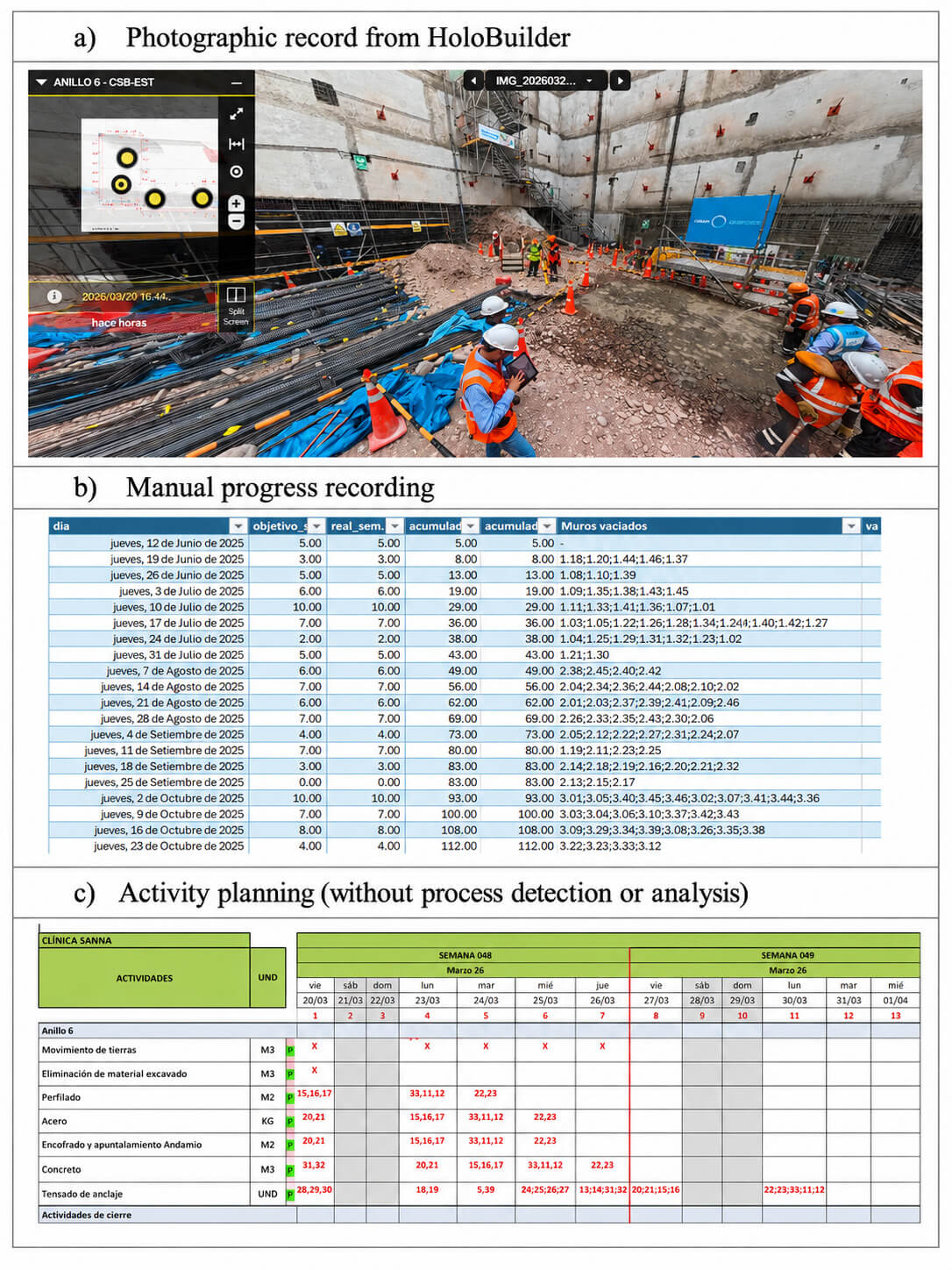
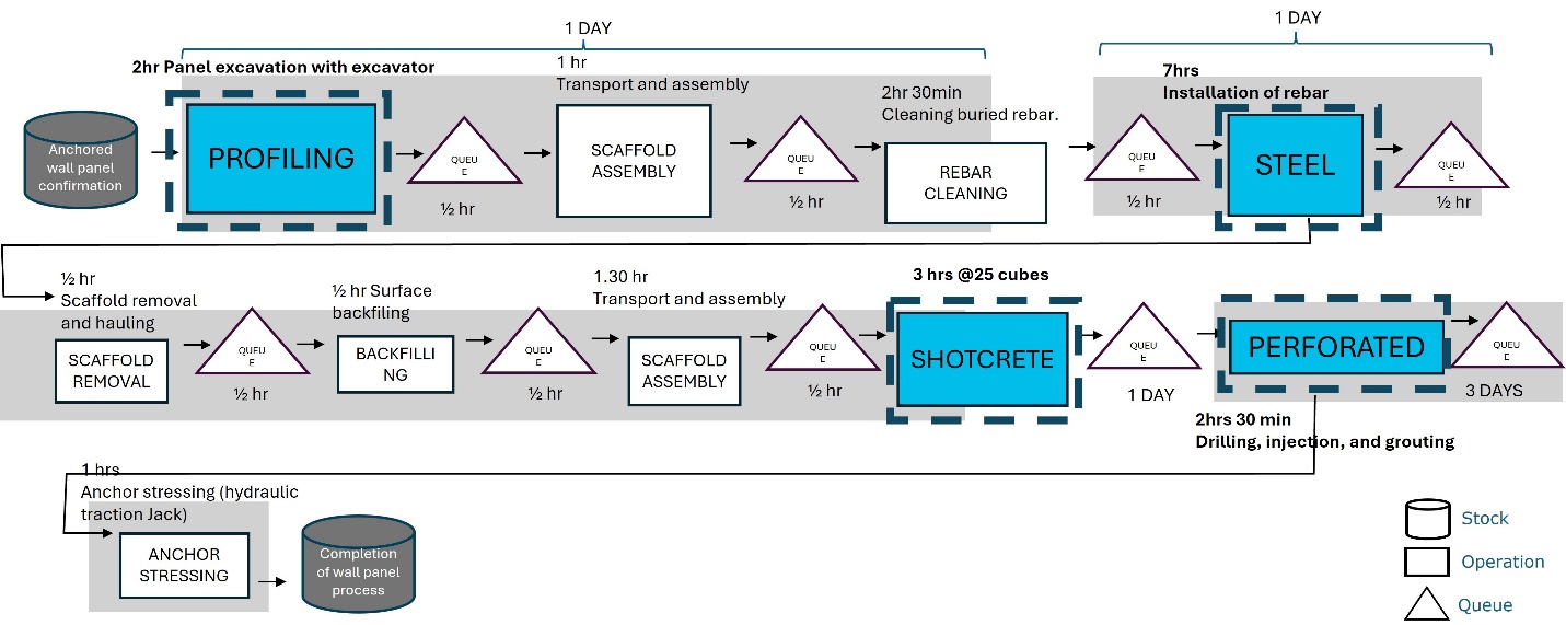
In anchored shotcrete retaining walls, the main sequence includes intermediate activities not always captured as primary work packages: manual finishing of profiling, scaffold assembly and removal, scarification, cleaning, inspection, manual filling, and preparation for shotcrete. These tasks consume time, space, and crews; they affect observed time by production state and can generate queues between stations.
The core gap is converting unstructured visual observations into auditable production events. A panel visually classified as steel may be under active installation, waiting, inspection, transition, or support work. Without temporal aggregation and production rules, these differences remain hidden. The research question is: how can field visual data be transformed into base variables for PPM metrics in anchored shotcrete retaining walls?
The wall panel is treated as the production unit. Its production system comprises four main stations: profiling, steel reinforcement, shotcrete, and perforation/anchoring, as well as precedence relationships, handoffs, queues, inspections, and support activities between stations. Under this representation, WIP corresponds to released or started panels that have not yet completed the cycle; throughput corresponds to completed panels per period; and cycle time corresponds to the time a panel remains in the system. In this study, the computer vision model focuses on the four main construction phases due to their duration, visual distinguishability, and schedule impact. Intermediate activities are included in the process map to represent the full production flow and may be incorporated as additional visual classes in future refinements when they are consistently observable in the field data. Fig. 3 presents the production system map for a single anchored wall panel.
The relationship between WIP, throughput, and cycle time, as expressed by Little's Law [2], serves as control logic rather than as a final measurement at this preliminary stage. If more fronts are released without sufficient capacity, WIP increases, queues accumulate, and cycle time extends. Production-state observability is therefore a prerequisite for constraint intervention.
Computer vision becomes useful when its outputs are aggregated by panel and region of interest (ROI). The ROI is the delimited area within the UAV frame that contains the wall panel and its immediate work zone, with panel extents derived from the BIM model, which provided the approximate length of each wall panel by sector and level (lengths varying by level); within it, EfficientNet-B0 classifies the visual state of the panel and YOLOv11 detects active crews. A single image is insufficient for production inference: each UAV pass over a panel produces multiple frames, from which the central frames are selected with the wall fully in frame; the flight log (GPS position and gimbal orientation) links each frame to the corresponding panel_id, allowing observations to be assigned to the specific wall the drone was observing at that moment. Table 1 translates PPM and Operations Science concepts into observable variables for anchored shotcrete retaining walls. In the Station row, phase_pred denotes the construction-phase label predicted by the EfficientNet-B0 classifier (profiling, steel, shotcrete, or perforation/anchoring), and phase_confidence denotes the softmax probability associated with that prediction.
| PPM / Operations Science concept | Definition in the retaining-wall system | Observable or computable variable |
|---|---|---|
| Production unit | Wall panel progressing through sequential stations. | panel_id, sector, level, ROI coordinates |
| Station | Main flow phase: profiling, steel, shotcrete, perforation/anchoring. | phase_pred, phase_confidence |
| WIP | Released or started panels that have not completed the cycle. | Count of active panels over time |
| Throughput | Panels completed per day or week. | Completion events per period |
| Cycle time | Time from release or first observed state to completion. | t_finish - t_start per panel |
| Queue / waiting | Panel ready for the next station but without the required active resource. | Time between the end of the previous phase and the start of the next phase |
| Constraint | Resource or station that accumulates queue and reduces output rate. | Upstream WIP + low release rate + increased waiting |
| Variability | Dispersion in durations, waiting times, and flow continuity. | Standard deviation, coefficient of variation. |
The proposed architecture is organized into four layers. Layer 1 captures data through UAV images and field video, linked to timestamp, sector, level, panel_id, and ROI. Layer 2 performs visual inference: EfficientNet-B0 classifies the construction phase of the panel, while YOLOv11 detects crew categories. Its outputs are class, confidence, count, dominant crew category (the crew class with the highest detection count in the ROI), and location. Layer 3 reconstructs production events using temporal smoothing, minimum permanence (the minimum number of well-framed frames per pass required for an observation to be registered as valid, guaranteed by the SOP flight protocol), and phase-crew-sequence correspondence rules. It distinguishes productive work, waiting, transition/support, inspection/release, interference, and candidate constraints. Layer 4 computes preliminary visual flow metrics: observed time by PPM state, observed time (s and %) by PPM category, temporal crew count, visual labor-time, and candidate-constraint signals. These outputs are the base variables for future continuous calculations of WIP, throughput, and cycle time. Fig. 4 summarizes the workflow from visual capture to preliminary PPM variables.
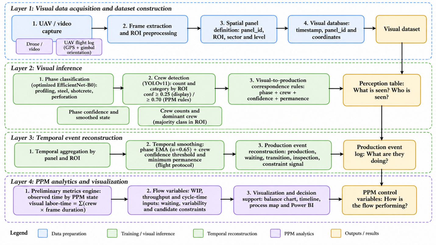
The methodology is structured around four operational questions. “What does the system see?” is answered through construction-phase classification. “Who does it see?” is answered through crew detection and counting. “What are they doing?” is inferred from the coherence among phase, crew, ROI, permanence, and sequence. “How are they doing it?” is evaluated through visual flow metrics computed from temporal events. Table 2 summarizes the relationship among operational question, system input, and expected output.
| Operational question | System input | Expected output |
|---|---|---|
| What does the system see? | Image or frame of the panel. | Construction phase: profiling, steel, shotcrete, perforation/anchoring. |
| Who does it see? | YOLO detections within the ROI. | Aggregated count and category of crews or personnel. |
| What are they doing? | Stable phase + crew + permanence + sequence. | Productive activity, support, transition, waiting, blockage, or probable rework. |
| How are they doing it? | Temporal events by panel and station. | WIP, throughput, cycle time, waiting, visual labor-time, variability, and constraints. |
A dataset of 13,706 real UAV images was used, distributed across four classes: profiling (3,317), steel (6,933), shotcrete/concrete (1,528), and perforation/anchoring (1,928) [7]. For balanced training, 4,800 images were selected (1,200 per class) with a 70%/15%/15% split for training, validation, and testing. The original distribution is unequal, steel exceeds shotcrete by more than four to one, because activities differ in duration and daily capture varied with construction progress; training with this imbalance would bias the model toward the majority class. The balanced subset eliminates that bias. The remaining 8,906 images were not discarded: they were reserved as an unseen real-domain set for domain shift analysis and uncontrolled post-training tests. Images were resized to 224x224x3 and augmented with geometric transformations, photometric variation, and Random Erasing [8]. Table 3 presents the original distribution, balanced subset, and data split.
| Class | Total images | Balanced set | Train (70%) | Val (15%) | Test (15%) |
|---|---|---|---|---|---|
| Profiling | 3,317 | 1,200 | 840 | 180 | 180 |
| Steel | 6,933 | 1,200 | 840 | 180 | 180 |
| Shotcrete | 1,528 | 1,200 | 840 | 180 | 180 |
| Perforation / anchoring | 1,928 | 1,200 | 840 | 180 | 180 |
| Total | 13,706 | 4,800 | 3,360 | 720 | 720 |
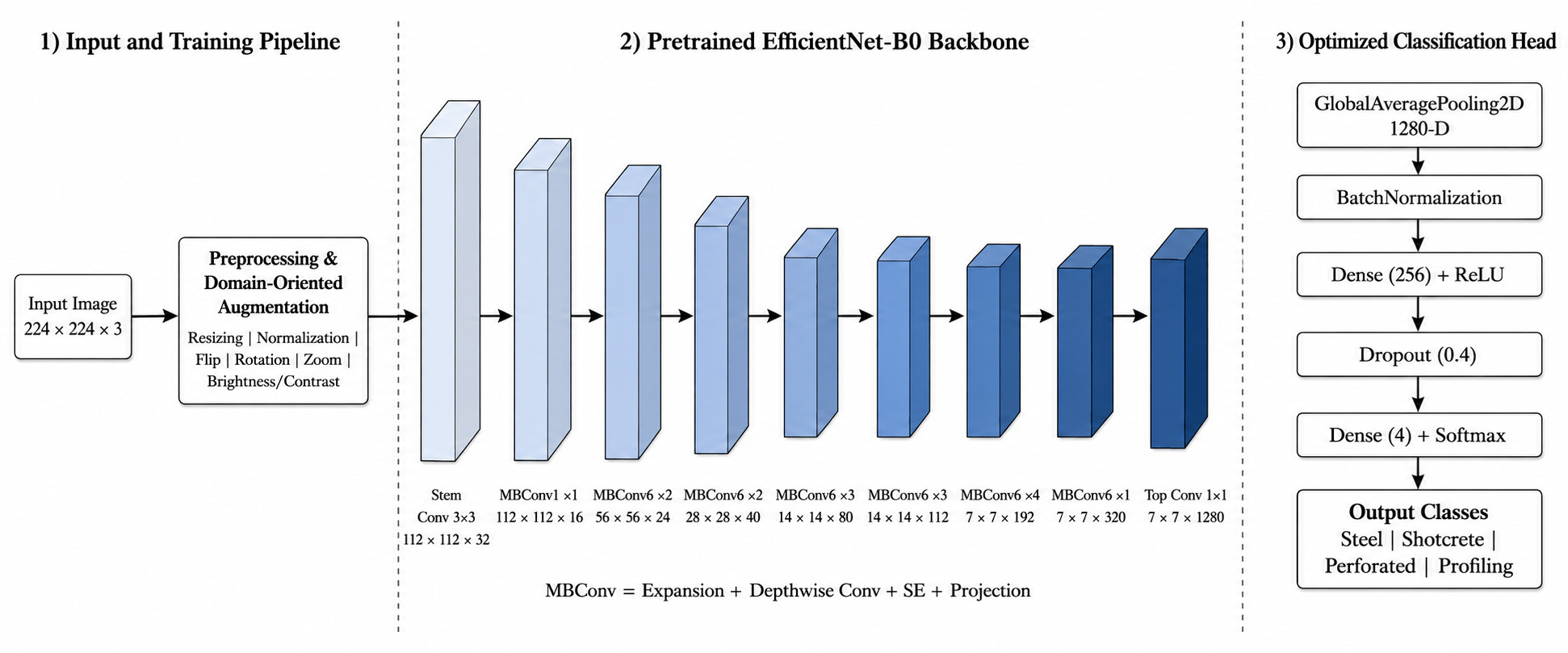
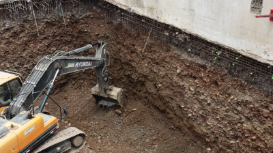
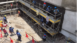
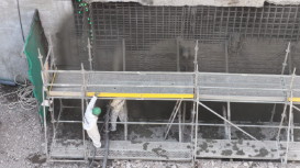
The classifier was implemented with EfficientNet-B0 pretrained on ImageNet. Transfer learning was applied by first training a four-class classification head with a frozen backbone [9], followed by progressive fine-tuning with decreasing learning rates on unfrozen upper layers. The optimized head included GlobalAveragePooling2D, Batch Normalization, a dense ReLU layer, Dropout, and Softmax output. Regularization and Random Erasing reduced dependence on shadows, scaffolds, and partial occlusions, frequent sources of domain shift in field images [10]. Fig. 5 presents the architecture and Fig. 6 shows representative examples of the real capture domain by phase.
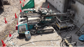
YOLOv11 was fine-tuned from pretrained weights (yolo11s.pt) using the same 13,706-image dataset, which already captures real site visual conditions including machinery, dust, occlusions, and diverse crews, without requiring additional data collection. Approximately 60% of the images (~8,200) were annotated with five crew categories: ironworkers (steel crew), masons (masonry/support crew), shotcrete crew, technical staff, and other workers. The first ~2,000 images were annotated manually; the remainder used model-assisted pre-labeling followed by manual correction. Training was conducted for 35 epochs (imgsz=960, batch=8, AdamW optimizer). The model produces bounding boxes, class labels, and confidence scores per detection. A confidence threshold of 0.25 is used for visualization; PPM inference rules require a crew detection confidence of at least 0.70. Lower values typically reflect partial occlusion by construction elements not represented during training. Each frame's output is interpreted as an aggregated signal of human resources within the ROI: presence indicates which crew categories are detected; density, how many members of each category; permanence, how long they maintain activity in the work zone. These terms refer exclusively to human resources; the system does not quantify materials or equipment.
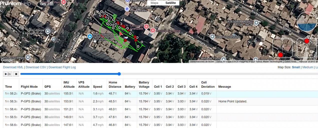
The dominant crew is defined as the crew category with the highest detection count within the ROI during the analyzed observation window [11]. Temporal aggregation is based on the UAV flight protocol: each drone pass over a panel produces a sequence of frames, from which the central frames are selected with the wall fully in frame and flight stabilized. The flight log, recording GPS position and gimbal orientation every second, assigns each frame to the corresponding panel_id. This resolves the key referencing challenge of using a mobile UAV instead of fixed cameras: the geometry of the deep excavation and the downward progression of the walls make a static camera impractical for covering all panels. Minimum permanence is defined as the minimum number of well-framed frames per pass required for an observation to be registered as valid; the SOP flight protocol guarantees this condition before an event is assigned to a panel.
Phase coherence is verified through the correspondence rules in Table 4.
Production-state inference combines phase, crew category, ROI, permanence, and sequence. If the panel is classified as steel and the steel crew remains active within the ROI, the event is interpreted as productive steel installation. If the panel retains the visual appearance of steel but no active crew is detected, it is classified as waiting or released panel. If the dominant crew is masonry/support, the event is classified as transition/support, associated with manual filling, cleaning, or preparation for shotcrete. If technical staff is present, the state is interpreted as inspection or release.
This logic prevents assigning all visually classified steel time to direct steel production. A single phase may contain production, waiting, inspection, transition, or interference. Table 4 presents the correspondence rules for converting visual observations into production events.
| Inferred state | Visual and temporal condition | PPM interpretation |
|---|---|---|
| Productive activity | Stable phase + expected crew + minimum performance in ROI. | The station is executed with a coherent resource. |
| Transition / support | Stable phase without confirmed change + support or preparation crew. | Work required to enable the next station without direct progress in the main phase. |
| Waiting | Panel ready + absence of expected crew or equipment during a defined window. | Queue or handoff failure between consecutive stations. |
| Blockage / constraint | Several panels accumulate waiting before the same station or shared resource. | A resource or station limits system throughput. |
| Probable rework / interference | Return to a previous phase, non-corresponding crew, or sequence inconsistency. | Deviation from planned flow requiring field review. |
Each observation is registered with timestamp, panel_id, predicted phase, phase confidence, crew count per category, dominant crew, ROI, and inferred PPM state. With this structure, KPIs can be computed at panel, station, and system levels. At this preliminary stage, WIP, throughput, and cycle time are architecturally enabled but require continuous, uninterrupted observation of the same panel from release to cycle completion. In the proof of concept, the metrics computable from the available clips are reported: balance chart by PPM category, temporal crew count, visual labor-time (crew count x frame duration), and process map. Table 5 summarizes the metrics and their interpretation for production control.
| Metric | Proposed calculation | Control interpretation |
|---|---|---|
| WIP(t) | Number of active and incomplete panels at time t. | Congestion and amount of open work. |
| Throughput | Completed panels / observation period. | Actual system output rate. |
| Cycle time | t_completed - t_released or first observed t_start. | Total residence time of a panel in the system. |
| Waiting time | t_start of next phase - t_finish of previous phase. | Queues, constraints, or coordination failures. |
| Transition time | Duration of support events between phases. | Work not visible in main work packages but relevant to flow. |
| Visual labor-time | Sum(crew count x duration x permanence x activity label). | Estimated visual effort by phase and state; not contractual labor-hours. |
| Cycle-time variability | Standard deviation or coefficient of variation of cycle time. | Flow stability and production reliability. |
| Candidate constraint index | Accumulated queue + low output rate + high station duration. | Prioritization of intervention on restrictive resource or process. |
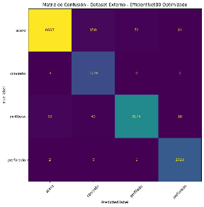
The optimized EfficientNet-B0 reached 97.15% accuracy and a macro F1-score of 0.9685 under evaluated real-site conditions. Class-level F1-scores were 0.9752 for steel, 0.9385 for shotcrete/concrete, 0.9671 for profiling, and 0.9930 for perforation/anchoring. These results validate the visual perception layer as a reliable input for production inference. Table 6 presents precision, recall, and F1-score by class.
| Architecture | Class | Precision | Recall | F1-score | Confusion Matrix |
|---|---|---|---|---|---|
| EfficientNet-B0 (Optimized) | Steel
| 0.9847 | 0.9660
| 0.9752
|  |
| Concrete
| 0.8888 | 0.9941
| 0.9385
| ||
| Profiling | 0.9775 | 0.9569
| 0.9671
| ||
| Perforated | 0.9877 | 0.9984 | 0.9930 |
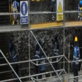
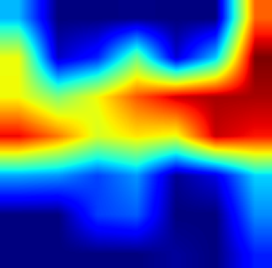
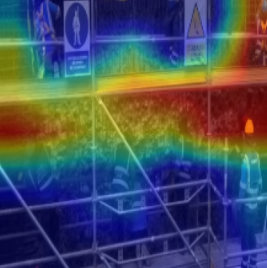
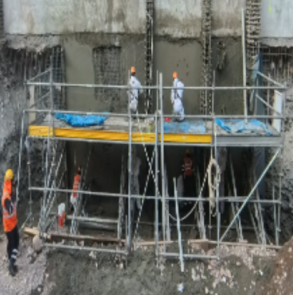
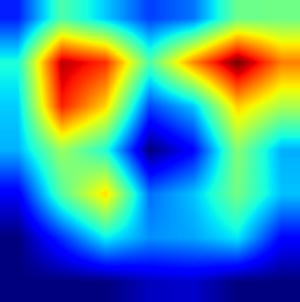
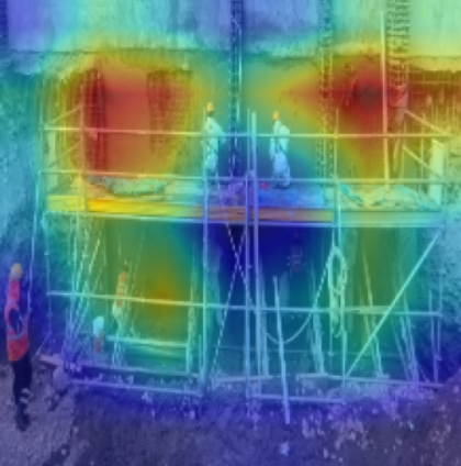
Grad-CAM maps were used to verify whether the model attended to visually relevant regions during classification [12]. In the evaluated cases, activations concentrate on installed steel, shotcrete surfaces, profiled ground, and perforation zones, confirming reduced dependence on non-causal visual context. Fig. 8 presents Grad-CAM examples under real field conditions.
The YOLOv11 detector complements phase classification by estimating crew presence and category. During validation, mAP50 stabilized above 0.95 and mAP50-95 approached 0.70, indicating sustained localization performance under complex visual conditions. Fig. 9 summarizes validation metrics, training losses, mAP evolution, and class-level performance.
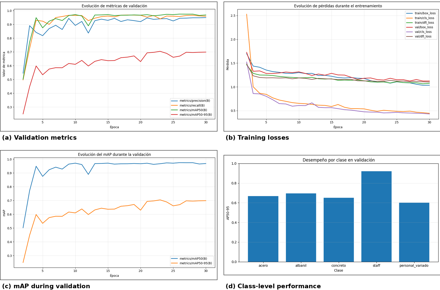
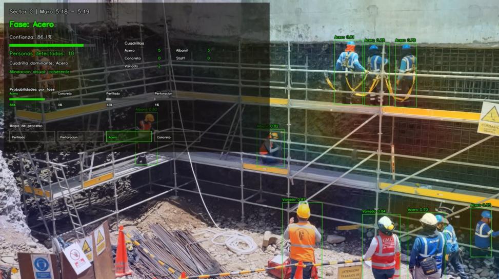
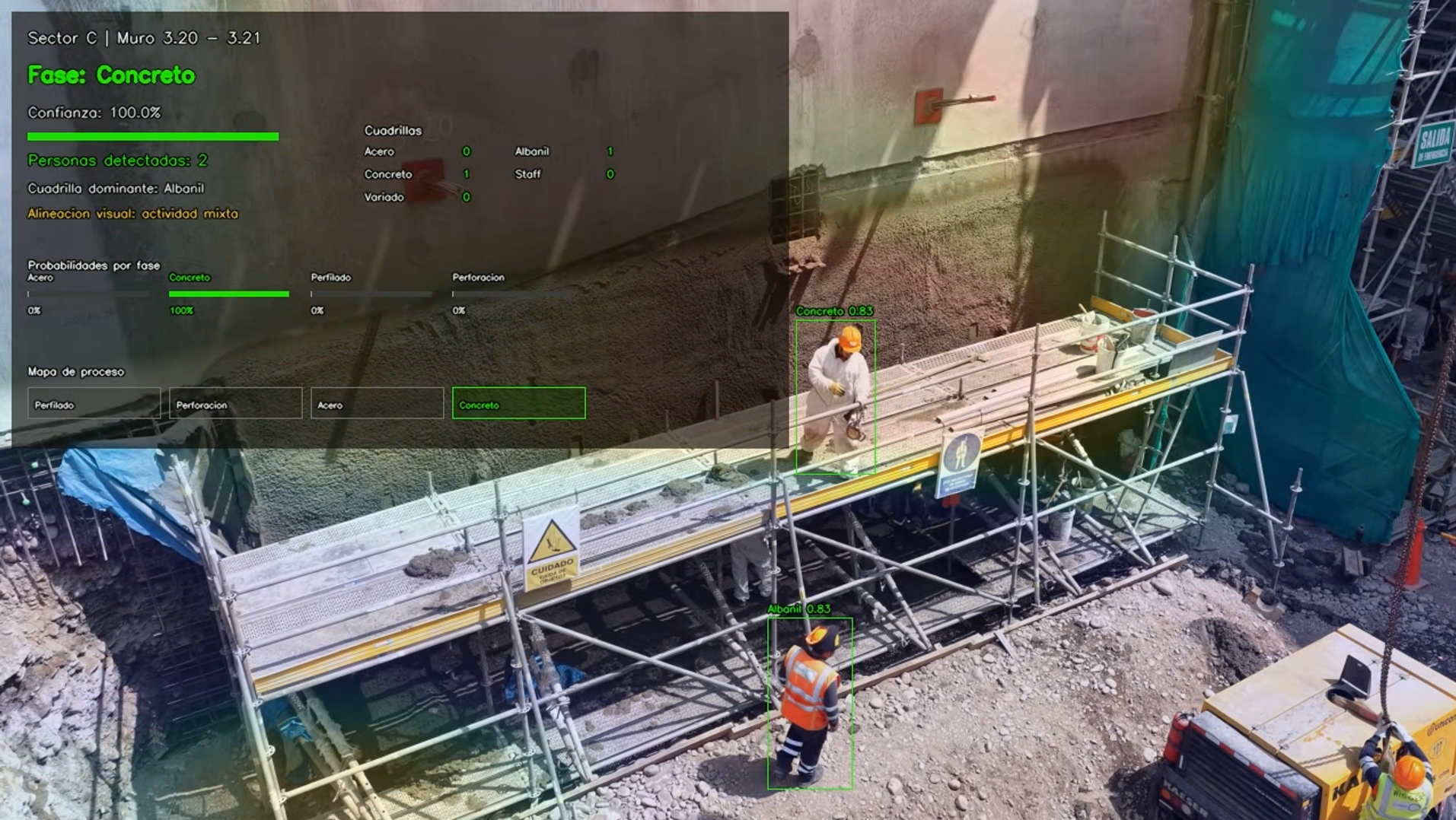
Fig. 10 shows visual inference examples in which the system identifies sector/wall, construction phase, confidence, personnel count, and crew category by ROI.
To evaluate the PPM layer, a representative steel-phase sequence was reconstructed from real UAV clips. The clips do not constitute a continuous recording of a single panel; results are therefore reported as proof-of-concept observed metrics, not as contractual cycle time, final productivity, or complete system measurement. The objective is to verify whether phase classification and crew detection outputs can be transformed into auditable production events.
Results show that the visual class “steel” encompasses distinct production states. With an active steel crew, the system infers productive installation. Without an active crew, it identifies waiting or a released panel. With masonry/support crew, it classifies the event as transition/support before shotcrete. With technical staff, it interprets the state as inspection/release. Table 7 summarizes the inferred production events in the observed steel-phase sequence.
| Segment | Dominant visual phase | Crew interpretation | Inferred PPM state | Observed time (s) | Production interpretation |
|---|---|---|---|---|---|
| Initial preparation | Prepared front / profiling | No active crew | Prepared / waiting | 25.0 | Prepared panel without active crew in the ROI |
| Initial steel assembly | Steel | Steel crew | Productive steel installation | 15.0 | Steel crew consistent with productive installation |
| Steel installation | Steel | Steel crew | Productive steel installation | 64.1 | Steel crew consistent with productive installation |
| Control / release | Steel | Staff / control | Inspection / release | 12.0 | Staff presence is consistent with inspection, control, or release |
| Post-steel waiting | Steel | No active crew | Waiting after steel | 40.0 | No active crew; possible handoff before next station |
| Pre-shotcrete support | Steel | Support / masonry crew | Transition / support | 22.0 | Support crew; possible manual filling or shotcrete preparation |
In the observed sequence, productive steel installation accounts for the longest duration, while post-steel waiting and transition/support represent non-production states that remain visually associated with the steel phase. This confirms that production flow cannot be characterized by visual phase classification alone; temporal aggregation and crew correspondence rules are required to differentiate these states.
The two active-steel segments, initial assembly and confirmed installation, are distinguished by the classifier's confidence level: at the onset of installation, part of the ROI still shows exposed excavation from the profiling phase and EfficientNet-B0 reports a steel-class confidence below 80%, reflecting partial panel coverage. As steel installation progresses and panel coverage increases, confidence exceeds this threshold and the system logs the phase as confirmed installation. The 80% threshold is the operational criterion used in this proof of concept to distinguish onset from full execution; it is not a contractual parameter. Table 7 does not represent cycle time for a single panel; it records the traceability between visual observation, correspondence rules, and production events.
Fig. 11 shows two contrasting cases during the steel phase: productive activity with a coherent crew and post-steel waiting without active crew.
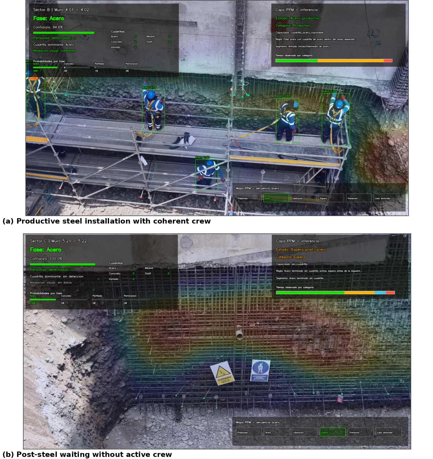
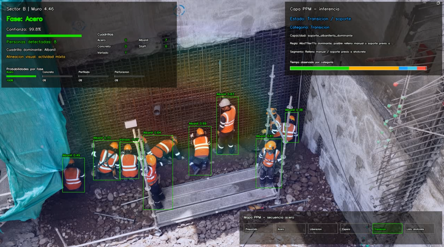
Fig. 12 shows a transition/support case in which the visual phase remains steel but the dominant crew corresponds to masonry/support work, compatible with manual filling or preparation before shotcrete.
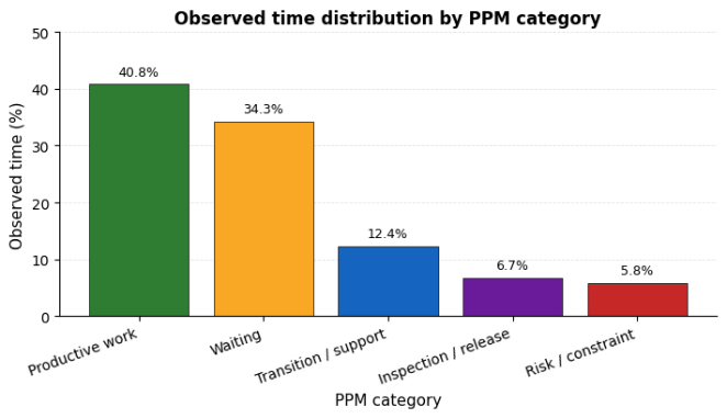
The balance chart summarizes observed time by PPM category: productive work, waiting, transition/support, inspection/release, and risk/candidate constraint. Temporal crew counts show changes in resource intensity and type. The process map shows that observed flow includes both direct production and enabling activities. Fig. 13 integrates the main PPM results from the observed sequence.
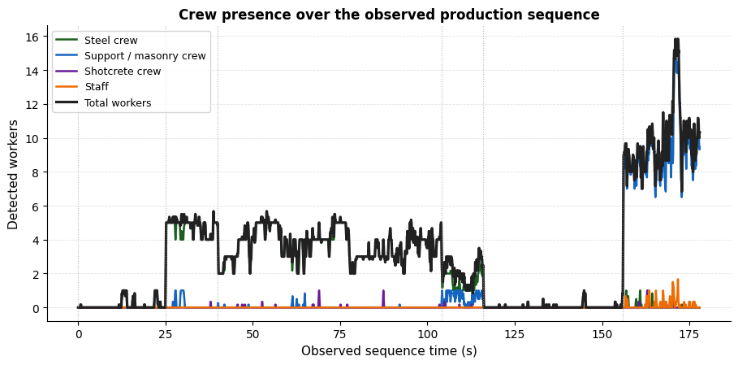
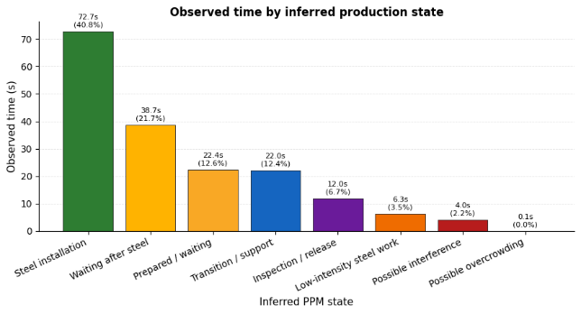
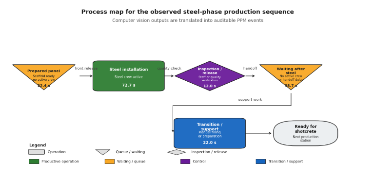
The proof of concept validates the framework's core premise: visual phase classification does not determine production state. A panel classified as steel can correspond to productive installation, post-steel waiting, inspection/release, or pre-shotcrete transition/support. Without phase-crew correspondence rules and temporal aggregation, UAV images document site conditions but do not produce flow data. The inference layer transforms those passive visual observations into discrete, auditable production events. The balance chart metrics demonstrate which base variables are computable from visual data. WIP, throughput, and cycle time are architecturally enabled but require continuous, uninterrupted observation of the same panel from release to cycle completion, a condition the present proof of concept does not satisfy given that the UAV clips are not continuous and activities may span more than one day. Importantly, the validated system architecture demonstrates that scaling to a continuously recording fixed camera would be technically viable, removing the dependency on UAV flight scheduling while preserving the same inference logic. Worker counts are indicators of resource intensity by production state, not contractual productivity or labor-hour measurements.
This study has four concrete limitations. First, the UAV clips used in the proof of concept are not continuous recordings of a single wall panel; results are demonstrative observed metrics, not contractual cycle time or final productivity. Second, UAV position variability, scale changes, occlusions, and viewpoint variation affect crew count consistency. Third, event assignment requires prior panel geolocation (ROI and panel_id definition), a manual step that must be standardized and automated for the system to scale to operational deployment. Fourth, the PPM inference rules are heuristics calibrated for this proof of concept and require quantitative validation by the production or project control team in any project where this type of solution is applied. Future work should focus on continuous panel-level observation through standardized UAV flights or fixed cameras where project geometry permits, persistent multi-object tracking, and quantitative validation of inferred states against actual production records, daily logs, and labor-hour data.
This paper presented a computer vision-based PPM framework for transforming UAV observations into auditable production events in anchored shotcrete retaining walls. The framework integrates four operational layers: visual data acquisition with UAV flight-log referencing, phase and crew visual inference, temporal event reconstruction, and preliminary PPM metric computation. The classification layer, built on an optimized EfficientNet-B0, delivers validated field performance: 97.15% accuracy and a macro F1-score of 0.9685 under real construction site conditions, with Grad-CAM maps confirming semantic alignment between model attention and construction-relevant features. The crew detection layer, based on YOLOv11 fine-tuned on annotated real-site images, complements phase classification by identifying five crew categories with a mAP50 above 0.95. The proof-of-concept application demonstrates that the same visual phase can contain structurally distinct production states, productive installation, waiting, transition/support, and inspection/release. This result validates the framework's central contribution: an auditable architecture that links visual perception with preliminary PPM variables, enabling the differentiation of production states that visual phase classification alone cannot reveal. WIP, throughput, and cycle time are computationally enabled by the architecture; advancing to full operational monitoring requires continuous panel-level observation and ground-truth validation against field production records, defining the immediate path for future research. The framework establishes the technical foundation for visual-data-driven production monitoring in deep excavation projects.