As a project progresses throughout its lifecycle, it is important for the project team to learn from prior completed activities in the system. This can be used to adjust the remaining contingency for the project. In this paper, this situation is modelled using Erlang Distribution. Using Bayes’ Law, the associated cost for the remaining work packages is adjusted and fit to the required confidence based on the updated arrival rates of the bottleneck resource.
Keywords: Bayesian Analysis, Erlang Distribution, Schedule

Bio coming soon

Ivan D. Damnjanovic is Professor and the Director of Engineering Project Management program at Texas A&M University. Dr. Damnjanovic specializes in qualitative and quantitative methods for management of engineering and project risks as well as management of infrastructure and transportation systems. He has an extensive experience in engineering r ...
In the history of project management, contingency has been a part of the project budgeting process as a flat line number, or a fixed percentage of the project estimate. Although this may work in some small project situations, it is important to consider all unique risks and challenges in each specific project to accurately quantify uncertainties. Unexpected challenges or delays can happen at any stage in the project lifecycle, adjusting the budget, scope, schedule, and therefore provides a need for contingency adjustments.
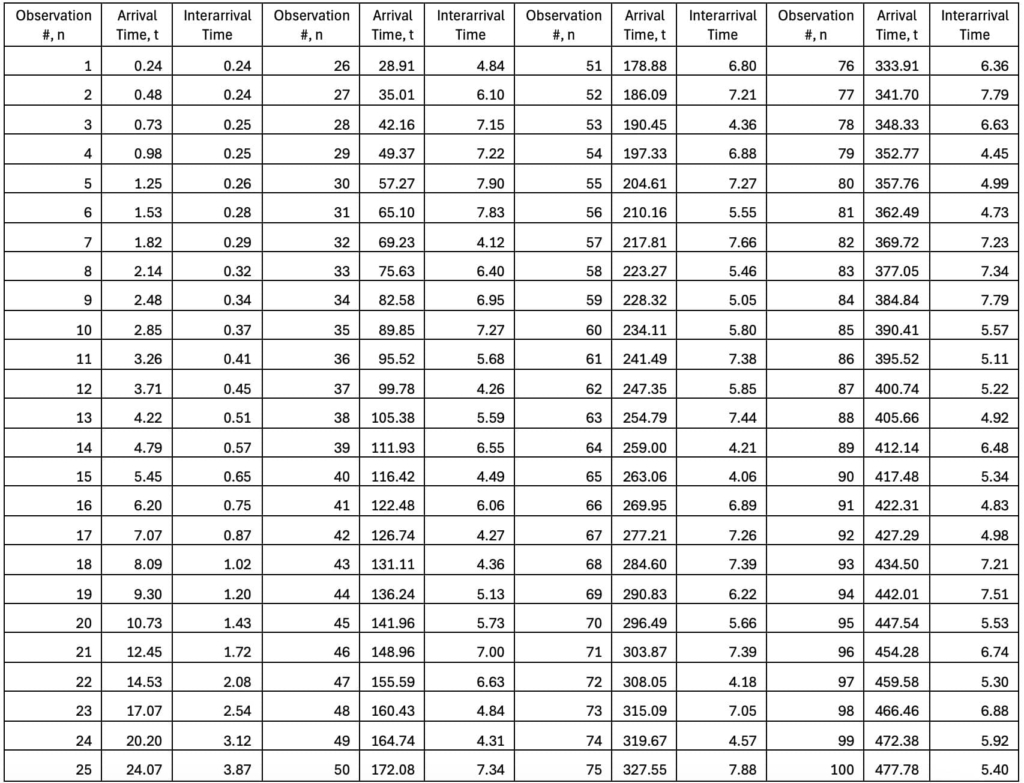
For modelling this process, a simple system is used to analyze the affect arrival rates of work packages have on the contingency. The system has three activities, C1, C2, and C3, each with differing service rates that are exponentially distributed. This is a pull system for activity C1 and the WP pushed downstream at a rate of 1 item per day. There are 100 work packages (N=100) in the system that need to be fulfilled.
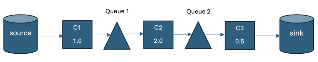
This situation is an example of a project production model with queues occurring between the activities when the processing time is smaller than arrival time. Activity C2 has a production rate of 2 items per day, and Activity C3 has a production rate of 0.5 items a day, or 1 item in 2 days. Simple models can be adopted for analysis of near-term production plans and 2 or 4 week lookahead schedules.
Because of the slower service rate, C3 determines the throughput of the system. This activity becomes the Bottle Neck Resource (BNR) with an average rate of 0.5 work packages per time, t (days). Hence, the throughput of the project is determined by this characteristic. The processing rate of the bottleneck resource, C3 is equal to the arrival of completed work packages. The raw process time is the time it takes a single work package to traverse an empty line, which for this system is RPT = 1 + 0.5 + 2 = 3.5 days.
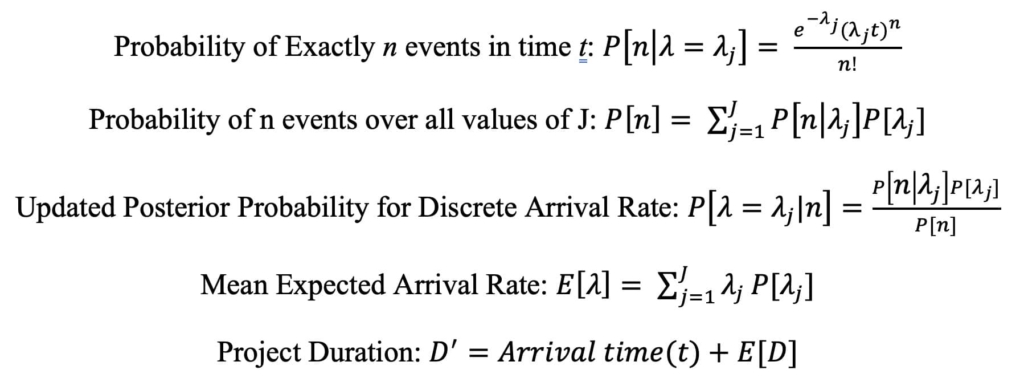
In this paper we are interested in setting up the project schedule contingency, in other words, we would like to know the distribution of the time to complete. The Erlang Distribution can be used to determine the expected rate until the 100th arrival. The Erlang Distribution is a generalized form of the Gamma Distribution that is used to model the time interval to the nth event. It is based on the Poisson, or constant rate process. It is defined by two parameters, k and μ, in which k represents the shape parameter that must be a positive integer, and μ being the scale parameter that must be a positive real number. The probability density function of the Erlang Distribution is:
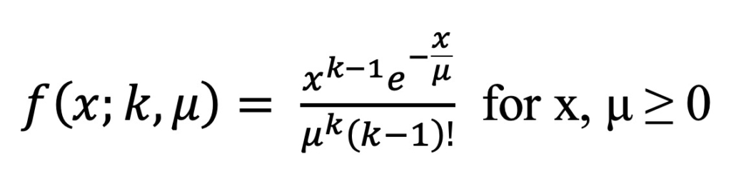
Figure 2 shows the Erlang Distribution, i.e. time to project completion for differing amount of work packages for our system throughput rate, 0.5 work packages per day.
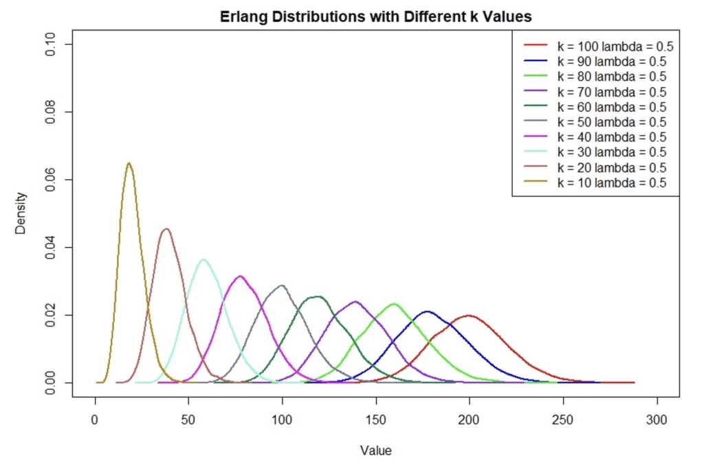
In our scenario, the k-value represents the number of work packages left to be completed in the project. The lambda value represents the estimated arrival rate that has been updated based on the observed data. As the k value converges to one, the probability for that instance becomes higher. Note that the Erlang Distribution with a k-value equal to one is the same as the Exponential Distribution.
Using Figure 2, one can easily specify contingency at various levels of confidence and remaining number of work items. Erlang, in this case, is very useful in determining the amount of time for the number of arrivals at question. In instance, when looking at k = 100 work packages with an arrival rate of 0.5 it logically makes sense for the distribution to center at 200. Although, when the arrival rates are constantly changing it gets a little trickier.
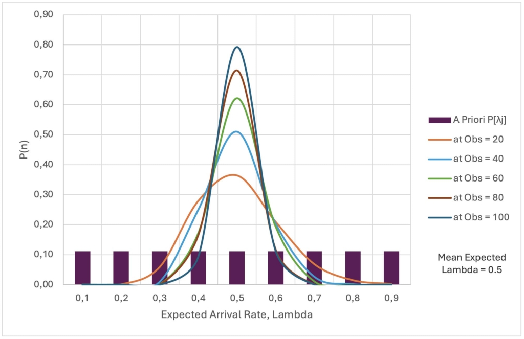
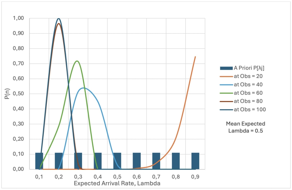
The throughput of the bottleneck is not always fully known before the project begins. At best, we have an estimate of that rate, sometimes based on historical data, and sometimes based on expert judgement. In this paper, we try to illustrate a situation where the initial BNR is defined with a mean rate of 0.5 with an uninformative prior distribution (uniform distribution).
We assume three different cases with arrival rates, or processing rate of bottleneck activity C3 ranging from 0.1 to 0.9 work packages per day with differing prior distributions per case. Using Bayes Law, the following equations are used to update the expected arrival rate after each work package is complete, which effects the total project duration. For this project, we want a contingency of P=80%. We use P=50% as an initial prior baseline project estimate with a static arrival rate value, as would be common in real-world construction projects.
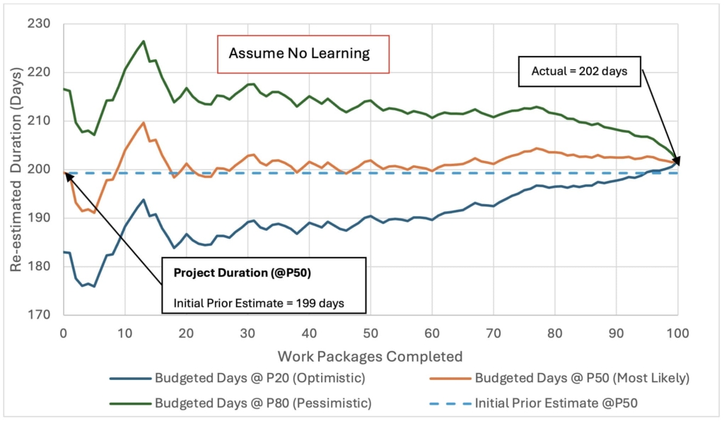
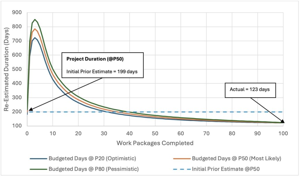
In this scenario, the arrival of work packages to activity C3 is random, aligning with our initial mean estimate of 0.5 work packages per day. Based on this, we assume a mean arrival rate of λ = 0.5 for our bottleneck activity C3 prior to project kickoff. This assumption is used to establish the initial budgeted duration, B0, of approximately 199 days, as depicted by the dashed line in Figure 4.
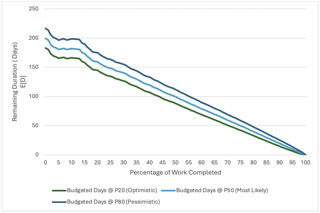
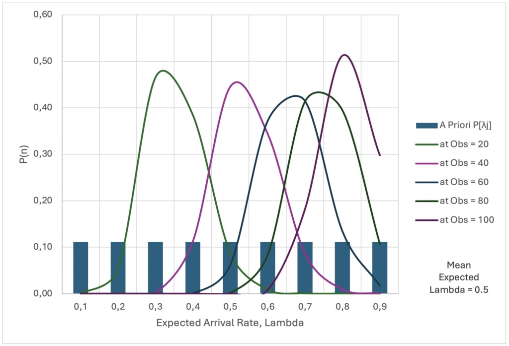
After each arrival observation, the expected arrival rate, E[λ], is updated based on the collected data. In this case, the updated project contingency closely matches the initial budget, B0, due to the minimal variance in arrival rates throughout the project and the accuracy of the initial λ estimate. As shown in Figure 5, the arrival rate stabilizes around 0.5 work packages per day after the first 20 observations, leading to a linear estimated project completion timeline, as illustrated in Figure 3.
With the completion of more work packages, confidence in the arrival rate of 0.5 increases, reaching nearly 80% by the end of the project. This consistency leaves an adequate amount of contingency throughout the project's duration, converging to zero as the project nears completion.
For Case #2, the crews experience a learning curve after the first eight arrivals. As they become more efficient, the arrival rate of work packages to C3 increases, as shown in Appendix 1. In this scenario, we look at two different prior mean arrival rate estimates in ALT A and ALT B. All arrival times remain the same in both alternates.
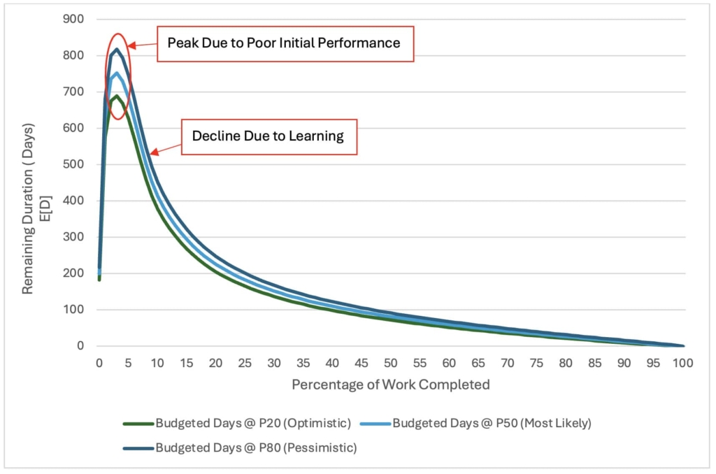
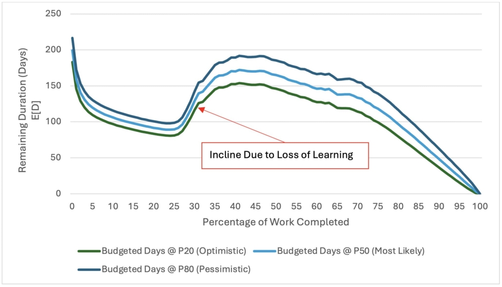
In Alternative A we again assume all arrival rates are equally as likely with a prior mean arrival rate before the start of the project of 0.5 work packages per day. This creates a baseline mean budget estimate of 199 days for project completion, prior to any activities actually starting. At the beginning of the project, the arrivals are much slower than previously predicting, with an expected cumulative mean around 0.16 work packages per day through the first 8 days. This is reflected in the upward spike shown in Figure 6. With the lower than predicted arrival rates occurring, the confidence in the remaining duration is lowered. After the first 10 days, the arrival rates began to drastically speed up, causing a sudden decline in expected project duration.
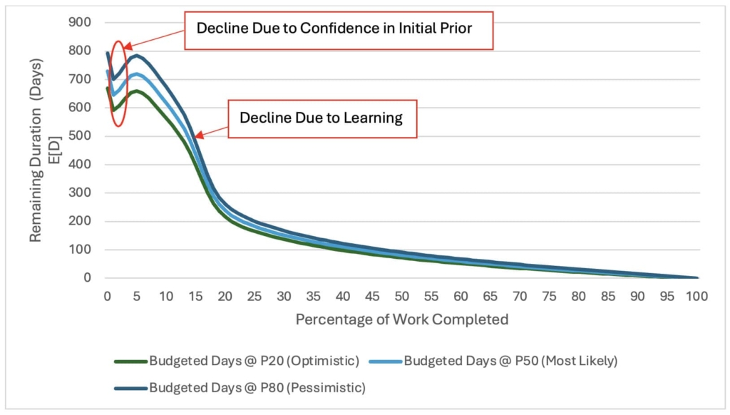
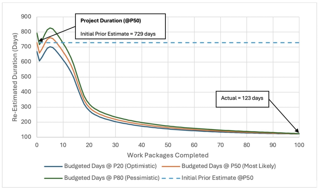
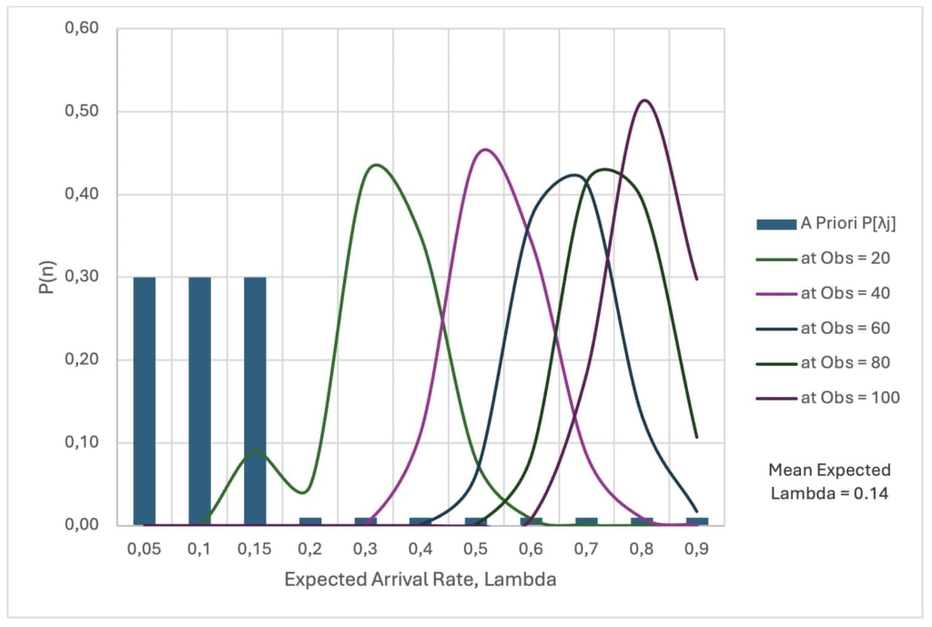
For Alternative B, the distribution of arrival rates is not uniform; rates of 0.05, 0.1, and 0.15 have a higher probability of occurrence based on previous data. Before project kickoff, we assume the mean arrival rate for our bottleneck activity C3 will be λ = 0.14 work packages per day. This estimate is used to create the initial budgeted timeline, B0, approximately 729 days to complete 100 work packages, as illustrated by the dashed line in Figure 7.
As the project progresses, the expected arrival rate, E[λ], is updated after each completed work package. Initially, there is a dip in the budgeted duration as confidence builds in the initial mean arrival rate estimate. However, as the arrival rate changes, the estimated budgeted duration increases again until stabilizing after the eighth work package. After the first eight work packages, the estimated project completion time is high, but as the crew learns and improves, the budgeted duration decreases significantly. As the posterior updates, the expected arrival rate values shift to the right. By the project's completion, the mean arrival rate is around 0.80 work packages per day, a significant improvement from the initial estimate.
This improvement allows for the release of more than half of the contingency by around the 25th day, freeing up resources that can be used in other projects or areas needing additional assistance.
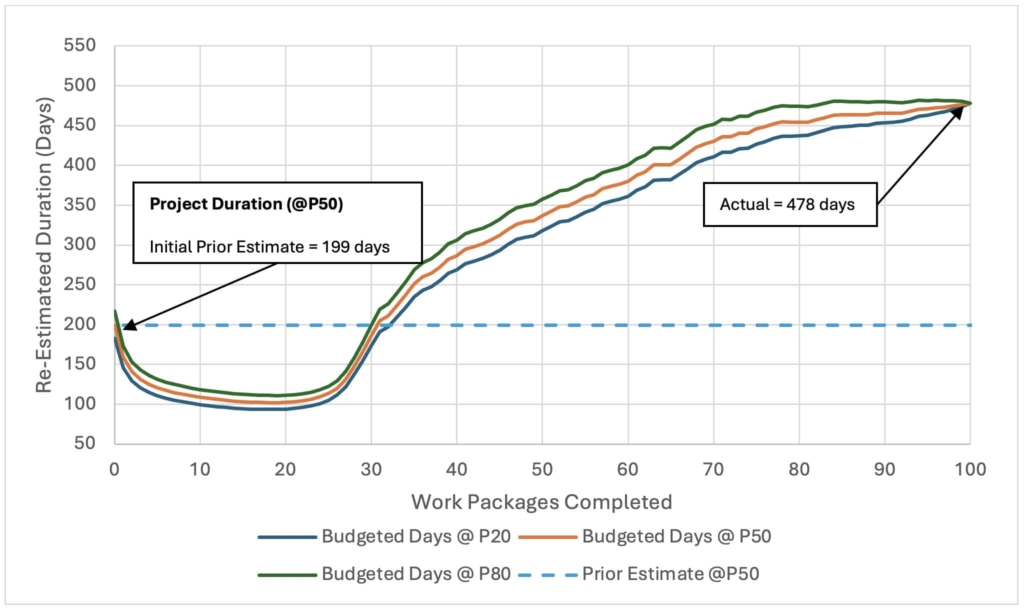
For Scenario #3, the initial estimate of the arrival rate to activity C3 is similar to that of Case #1 and Case #2 ALT A, at λ = 0.50 work packages per day. The initial budgeted timeline, B0, is approximately 199 days to complete 100 work packages, as illustrated by the dashed line in Figure 10. However, as the project progresses, the arrival rate decreases from the initial estimate and continues to decline for the rest of the project.
This is the opposite of what occurs in Scenario #2. In this scenario, the initial estimate creates false optimism about the project's total duration, which ultimately proves detrimental. By the end of the project, the mean arrival rate is found to be around 0.2 work packages per day, significantly lower than the initial estimation.
Without updated contingencies, the project would significantly exceed the budgeted duration. However, since the arrival rates are updated after each completed work package and the budget is dynamic, the project manager remains aware of the situation. This allows the project manager to allocate additional resources to prevent project failure.
For each case of the same system, the contingency widely varies. For Case #1, the estimated budget and observed budget with 80% confidence are similar due to the close approximation of the arrival rate at Activity C3. Although, that is not the illustration of Case #2 or Case #3.
For Case #2, in both alternatives the project's contingency allocation was excessive due to a conservative initial estimate of arrival rates. As the project progressed and the arrival rates improved due to the learning curve of the crew, a substantial portion of the contingency budget became unnecessary. This surplus could be reallocated to other project needs or reduced to optimize overall resource utilization. It is important to note around day 20, the estimated remaining budget became similar regardless of the initial prior estimate of arrival rate.
Conversely, in Case #3, the initial overestimation of the arrival rate led to an underestimation of the necessary contingency budget. As arrival rates decreased over time, the project risked significant delays. However, by continually updating the arrival rate estimates and adjusting the contingency budget, the project manager is able to anticipate these delays and take corrective actions, such as reallocating resources or adjusting the schedule, to avoid project schedule failure.
These cases demonstrate the critical role of dynamic contingency management in project success. Traditional approaches to project management often employ static contingency measures, disregarding the dynamic nature of project environments. By employing statistical methods like the Erlang Distribution and Bayesian updating, project managers can make informed decisions based on the most current data.
In an era where projects are becoming increasingly complex and subjected to various uncertainties, the ability to dynamically adjust budgets based on real-time data becomes indispensable. The integration of these statistical methods into project management practices not only improves the accuracy of project duration estimates but also enhances the strategic allocation of resources, ultimately contributing to the overall success and efficiency of projects. This cuts out unnecessary variability and uncertainty found in project estimates.
By examining different scenarios with varying initial estimates and arrival rates, this paper illustrates the benefits of a dynamic approach to contingency management. The results emphasize the importance of flexibility and adaptability in project planning, enabling project teams to respond effectively to changes and uncertainties becoming more resilient in nature. As project management practices continue to evolve, integrating statistical methods and real-time data analysis will be essential for achieving more accurate and reliable project outcomes.
Future work for this paper will focus on significant enhancements to the current model. One key area for development is the incorporation of cycle time and Work-In-Progress (WIP) metrics to more accurately assess quality risk. Additionally, extending the model to accommodate more complex production systems would provide a more comprehensive understanding of diverse construction environments. Another addition is defining processing time using different statistical distributions, which would allow for a more representations of variability in the project cycle. Lastly, addressing moving bottlenecks within the model could lead to more dynamic and responsive optimization strategies, ultimately improving the overall efficiency and robustness of the project system.
Albert, Jim. “LearnBayes: Functions for Learning Bayesian Inference.” Rdrr.Io, May 2019, Accessed May 2024.
Damnjanovic, Ivan. “Bayesian Revision of Probability Estimates.” Lecture 12. Lecture 12, Apr. 2024, College Station, TX.
Damnjanovic, Ivan. “On Managing Contingency and Budget to Complete.” Lecture 13. Lecture 13, Apr. 2024, College Station, TX.
Damnjanovic, Ivan. “Overview of Project Risk Management.” Lecture 5. Lecture 5, Jan. 2024, College Station, TX.
Gosavia. Tutorial for Use of Basic Queueing Formulas, https://web.mst.edu/~gosavia/queuing_formulas.pdf.
Hopp, W. J. (2011). Supply chain science. Waveland Press.
Ibe, O. C. (2013). Markov processes for stochastic modeling ed. 2. Elsevier Science.
Jacobs, Marc. “Statistical Rethinking — Bayesian Analysis in R.” Medium, 6 Dec. 2021, https://medium.com/@marc.jacobs012/statistical-rethinking-bayesian-analysis-in-r-e1e25aeb9a5c.
Jiménez, P., Cañadilla, & Montoya, Y., Román. (2017). Queueing: A package for analysis of queueing networks and models in R. The R Journal, 9(2), 116. https://doi.org/10.32614/rj-2017-051
Massachusetts Institute of Technology. (2011, Spring). Chapter 2 - Poisson Processes. Discrete Stochastic Processes. https://ocw.mit.edu/courses/6-262-discrete-stochastic-processes-spring-2011/3a19ce0e02d0008877351bfa24f3716a_MIT6_262S11_chap02.pdf
Shortle, J. F., Thompson, J. M., Gross, D., & Harris, C. M. (2017). Fundamentals of queuing theory. John Wiley & Sons, Inc.
Wang, Kuo-Hsiung, and Keng-Yuan Tai. “A queueing system with queue-dependent servers and finite capacity.” Applied Mathematical Modelling, vol. 24, no. 11, Sept. 2000, pp. 807–814, https://doi.org/10.1016/s0307-904x(00)00013-5.
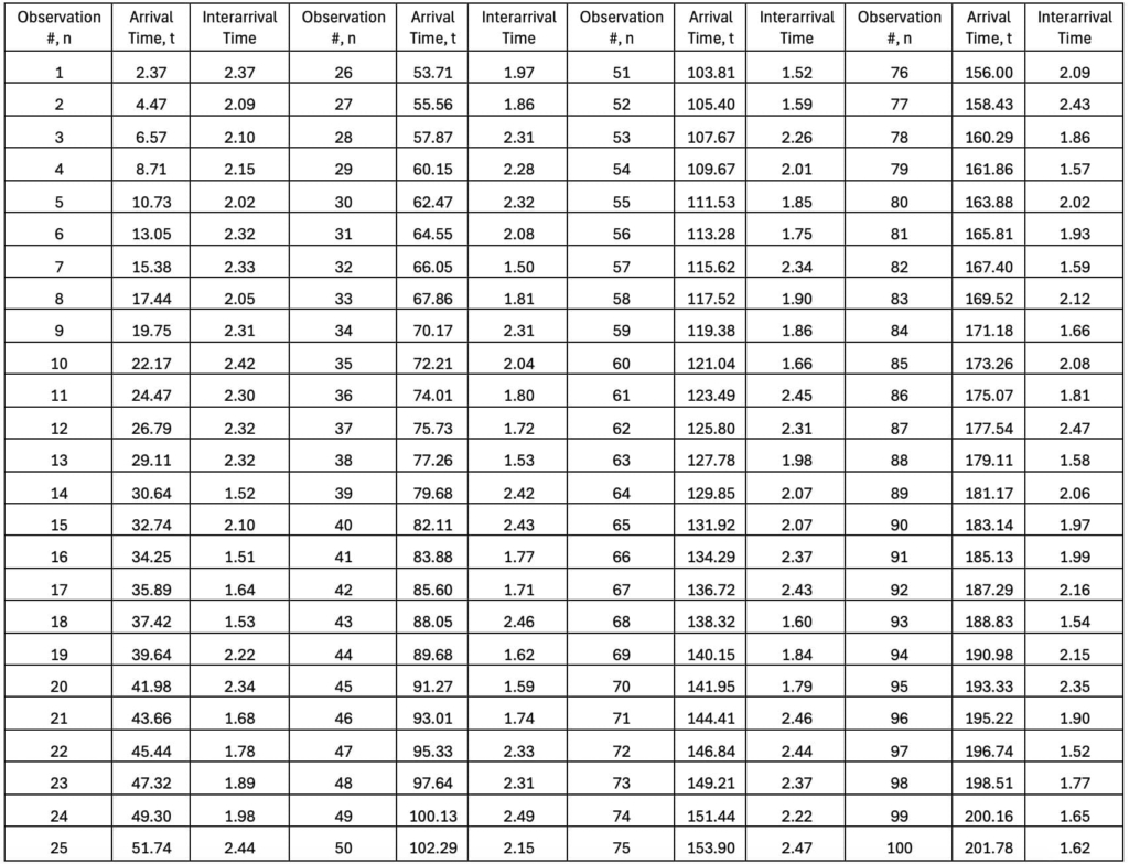
Case1 Data
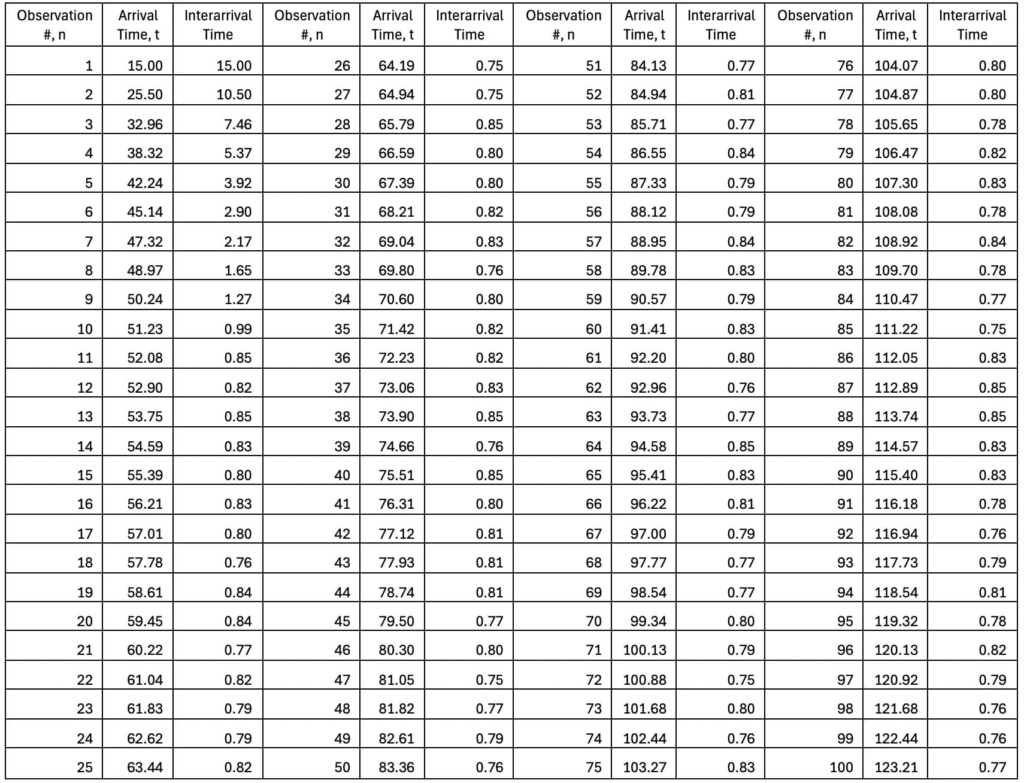
Case 2 Data
Case 3 Data