More Robust, Insightful And Faster Production Modeling Through The Integration Of Discrete Event Simulation With Analytical Modeling

Introduction

Achieving predictable schedule and cost, without changing the scope, and while meeting the desired health, safety, environmental and quality standards, has been, and continues to be, an objective of constant pursuit by owner/operators, contractors, vendors as well as academics and solution providers. To do so, many rely on building a model that describes either what needs to happen or predicts what might happen using common project management approaches. Modeling what needs to happen typically utilizes deterministic models such as Critical Path Method (CPM) or Gantt Charts, whereas modeling what might happen may utilize stochastic approaches such as Program Evaluation and Review Technique (PERT) that uses weighted averages of optimistic, pessimistic, and most likely estimates of task duration to predict total project duration. Monte Carlo schedule simulations that leverage many iterations of random sampling to generate a probability distribution of possible project durations are also used.

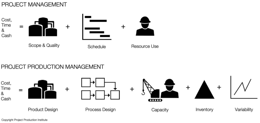
Although these deterministic and stochastic approaches have been around for more than half a century, recent reports on project performance still show predictable project results are difficult to achieve. The root causes for this phenomenon and what can be done to address has been the source of many academic research and industrial movements including AWP, Lean Construction, Agile in Construction, etc. However, from the Project Production Management (PPM) perspective, this lack of performance is due to looking at the cost, time and amount of cash tied up during a project as a function of scope & quality, schedule and resource rather than focusing on the five levers of production system optimization, where cost, time and amount of cash tied up are a function of product design, process design, capacity, inventory and variability (Figure 1).

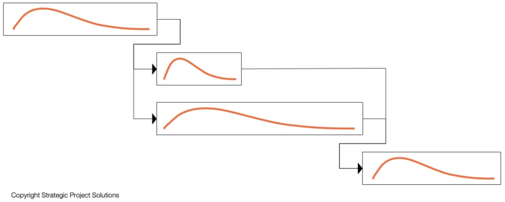
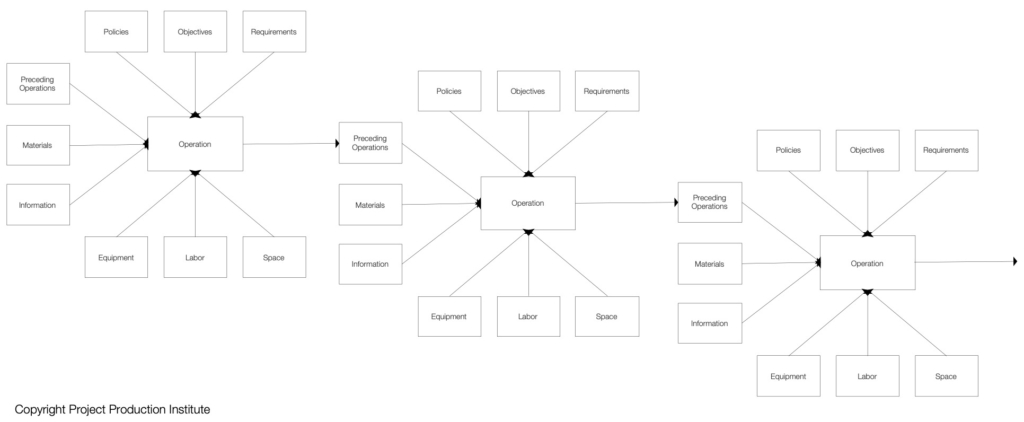
This thinking is reflected in the current way of modeling, where schedule activity durations are used to account for all types of variability regardless of the sources (Figure 2). Most of the Monte Carlo simulations currently used in the construction industry follow this approach. Regardless of the number of runs and how well the durations from past projects are captured, due to the lack of expressiveness in describing the interaction between the activities and the resources, especially shared resources (e.g., a single resource does work for two or more tasks), the output cannot only be misleading, but provide very little room for optimization other than how to reduce the duration itself or the associated variations. Interestingly, this brings the focus back to how the work is done, i.e., the 5 levers of PPM.

However, as described by Operations Science, the duration on an activity is not just a summary of how long the operations within the activity take, but also a function of how long things wait to be worked on. Waiting can occur due to labor, equipment and/or space being occupied working on something else (queue time), or batch being formed (batch time), or lack of matching items for assembly (wait-to-match time), etc. To see a full list of reasons for “waiting”, refer to Choo & Spearman (2019). Many of these reasons for waiting are external to the operation itself and are driven by the behavior of the resource that is performing the work as well as how big a chunk of the work is provided at once. Therefore, reflecting these behaviors as a statistical distribution of task duration is misleading.

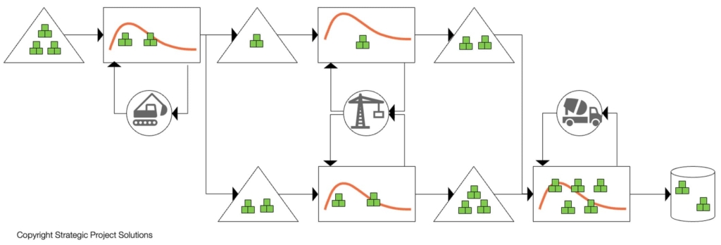
To address these issues, academics have been proposing the use of discrete event simulation (DES) to model project operations for more than 60 years (Teicholz 1963, Martinez 1996, Tommelein & Ballard 1997), where the interaction between the available of the prerequisite work and the resource that perform the work can explicitly determine whether the work can begin (Figure 3). Despite its wide applicability and usefulness, it is still yet not widely adopted in the industry as it requires both understanding how the work is done, i.e., production aspect of the project, and how to build and analyze the model. As for the latter, and as can be seen in a very simple model in Figure 3 above, building a DES model that describes, and closely resembles reality, is very time consuming. In addition, it takes a long time to optimize when there are many variables, resulting in a very large number of combinations of possible scenarios. Nevertheless, it is a great solution to figure out what may happen when the production system is “turned on” based on the current targets and plan. Although this is how DES is used by many, it becomes a little trickier when it is used to determine what the potential opportunities are to optimize the production system.

To illustrate, let’s assume we want to determine the right amount of construction equipment to deliver a project on time and how much work-in-process ensures cycle time is within acceptable range. If we consider a process with five types of equipment with each equipment count being somewhere between 1 to 5, that equates to 125 (= 5x5x5) different scenarios. At the same time, if WIP is somewhere between 5 – 50 units (e.g., panels, modules, systems, zones, areas, rooms, etc.), that represents 46 alternatives. Combining the two means we would have to analyze 5,750 different scenarios. Furthermore, and since each operation has variability, let’s assume each scenario needs to be run 100 times to create a statistical output that can be used to determine what the average and standard deviation for the overall project duration is. This now results in 575,000 simulation runs. Assuming each run takes one second (since the process is simple), it would take roughly 6.6 days non-stop to run all scenarios, if the simulation engine runs consecutively. To minimize this issue, there are techniques that have been used to prune the number of alternatives that needs to be run, but that requires outputs to be analyzed either automatically or manually before some of the alternatives can be eliminated. To minimize the time it takes to run all the scenarios of complex models with many parameters often leverage powerful computers with parallel processing capability. However, many modelers with only regular laptop and desktops may still leave the computer running overnight (or longer) so that the results can be analyzed when it is done. If the simulation fails, it quite often results in having to re-run the simulation all over again.

One very powerful and effective way of alleviating this challenge is to use an analytical model, when possible, to determine what the optimal values are or rapidly expose potential areas for optimization. Since analytical modelling uses mathematical expressions to describe the behavior of a production system, it can be “solved” rather than “simulated” for insights and optimization much faster compared to DES. Since there are certain limitations on where analytical model can be applied, combining the two approaches enables a more robust, insightful and faster result.

Comparison of Modeling Approaches

Before diving into each approach, we should exemplify what “model” and “simulation” mean. Although there are many definitions of these terms in the Merriam-Webster Dictionary, most relevant definitions for this paper are “to produce a representation or simulation of” for model, and “the imitative representation of the functioning of one system or process by means of the functioning of another” for simulation.

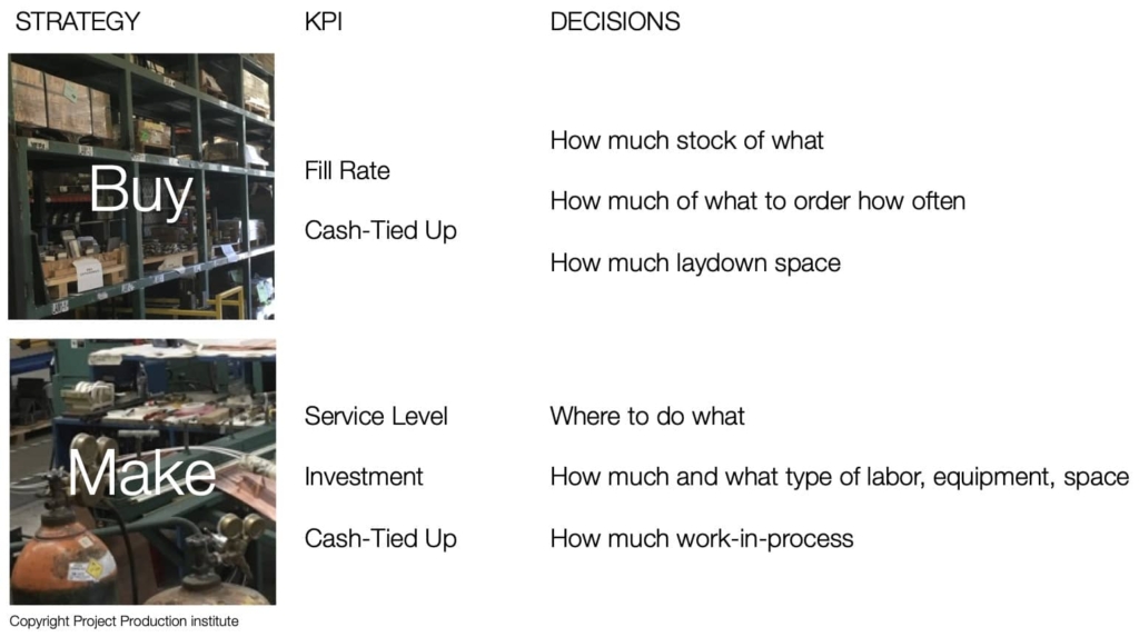
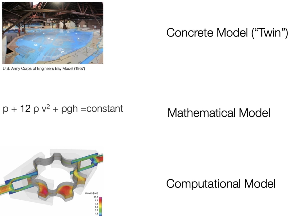
This definition begs the question what behaviors a model should imitate, and which questions should it be able to answer? Table 1 shows some of the key questions that a model should be able to answer or assist in answering depending on whether "it" is being produced internally or provided by others. Although there are many options such as administrative processes, contracting relationships, communications, etc., the author believes modeling the production aspect of engineering, fabrication, delivery, installation and commissioning including associated supply network, provides the best form to improve project performance including time, cost and cash flow. So, what type of modeling approach, including what parameters, best suits, imitates the behavior of project production systems? Figure 4 shows common forms of models used in construction and manufacturing. Although some of these forms include physical models, these are becoming digital models, a.k.a., “Digital Twins” and “Virtual Twins”, due to the proliferation of modeling tools and powerful computers.

Another type of models is mathematical models. They can be broken into two subtypes: (1) analytical models and (2) numerical models. Analytical models are used when there is a well-defined solution allowing exact answers to be calculated. Numerical models are used when there is no exact solution and are solved using more of a trial-and-error approach until a “good enough” answer is achieved. Most of the machine learning models can be categorized as numerical models.

On the other hand, computational models leverage computers to analyze and simulate systems. Their applications span many industries including construction and manufacturing. One example of a computational model in engineering and construction is Computational Fluid Dynamics (CFD) as in Figure 4 that is used to design fluid systems including air, water and chemical. Computational models can mainly be categorized as: (1) Agent-based, (2) Continuous and (3) Discrete Event.

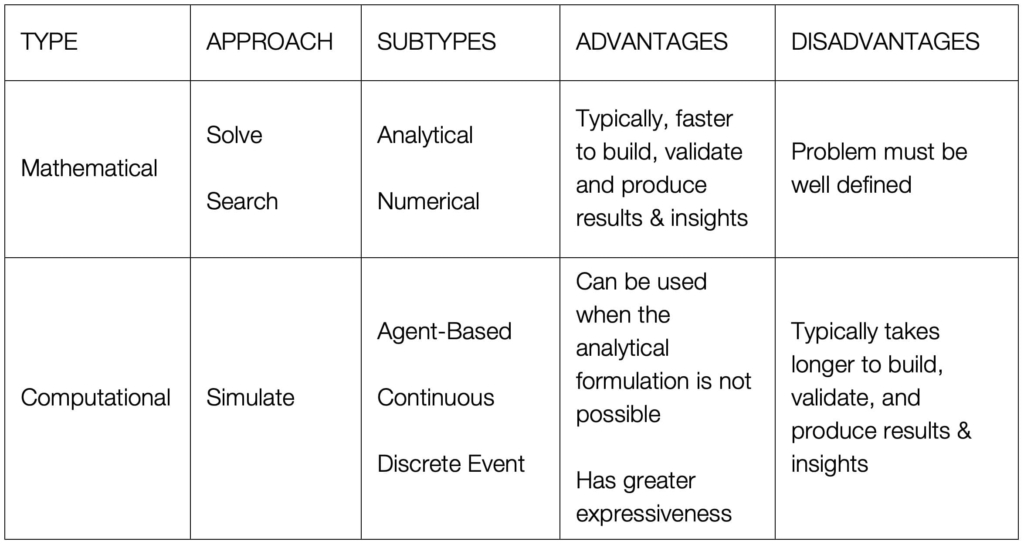
Agent-based models are used to understand the behavior of a system through the interaction between agents (people, things, etc.) For example, agent-based systems have been used to design effective entries and exits of a building by simulating the behavior of people in non-emergency and emergency situations at various levels of capacity. Continuous simulation models are used to understand the state of a system that changes continuously (e.g., Computational Fluid Dynamics). Discrete event simulations are used to analyze the state of a system that changes at the start or end of events. Table 2 summarizes the comparison between mathematical and computational modeling approaches.

Based on the characteristics of these modeling approaches, analytical modeling and discrete event simulation provide the most effective and efficient means to leverage Operations Science to analyze, simulate and optimize production systems. Which one to use when may depend on characteristics of the production system. In certain conditions (to be examined later), analytical models alone should provide sufficient insights to analyze a production system. In other conditions, analytical models may not be sufficient, and therefore, must rely on DES as well to gain additional insights. However, just relying on DES to optimize a production system can result in frustration due to the amount of time spent on running and testing non-optimal scenarios.

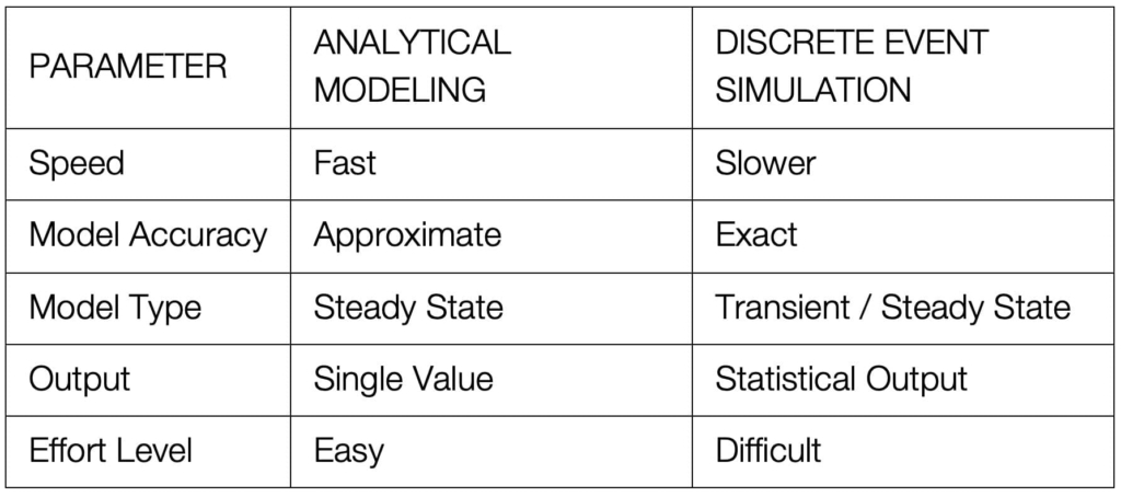
Let’s examine the characteristics that make one approach more applicable than others. Since an analytical model is a mathematical model that is solved, it is typically much faster to execute than a DES model. However, as with any math problem, the parameters cannot change while the problem is being solved. Therefore, analytical model assumes a steady state. This does NOT mean analytical models can only apply to situations without variability. Analytical models can incorporate demand variability, process time variability, batch size variability, etc., however, it means the behavior of the system do not change over time. Since this constraint does not apply to discrete event simulations, DES can be used in transient states as well. However, they typically take longer to build and run than equivalent analytical models. Table 3 summarizes the applicability of the two modelling techniques.

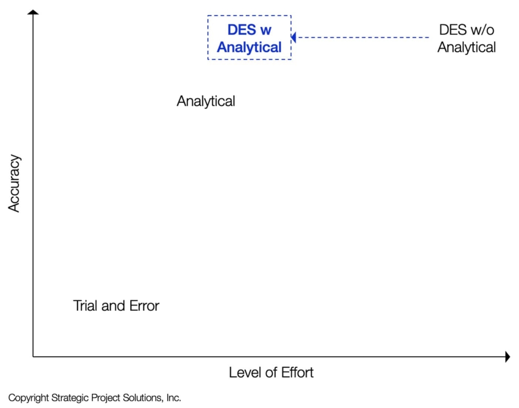
If the speed of the analytical model can be used to provide a starting point for a DES study, it would greatly reduce the amount of effort required to generate an optimal solution (Figure 1).

Analytical Modeling

Since an analytical model is a numerical model where the solution is solved rather than simulated, formulas provide insights into what parameters are required to structure a real-world problem into a model. This is highly valuable as this answers the question: “what data is needed to model the production system?” The formulas from Operations Science such as the ones in Figure 6.

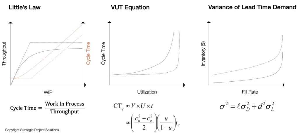
For example, one of the structures used to describe a production system is “process step” with parameters such as average and standard deviation of the process rate, average and standard deviation of the setup time, resources that are used to perform the work, as well as yield and setup cost for the process step to name a few. This is tremendously useful since it assists project teams in understanding what data needs to be collected / extracted from existing data sources such as schedules, estimates, budgets, bills of material, etc.

When applied to production systems, analytical modeling can produce highly insightful results as explained next.

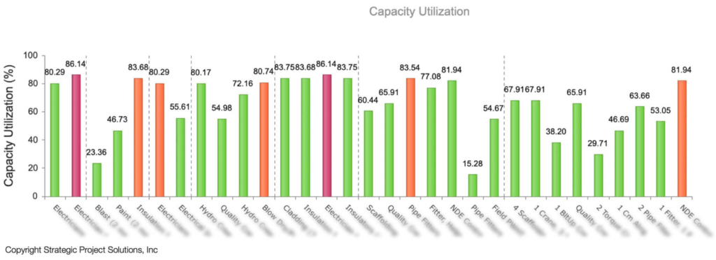
Average Capacity Utilization (Figure 7) is calculated as demand / capacity where capacity is defined as the maximum throughput of a given resource and is a function of what mixture of items (pipes, modules, drawings, etc.) are flowing through the production system in a particular batch size, and the demand, defined as the sum of all workloads that must be performed by the resource. The resource with highest average capacity utilization is the bottleneck. Since the demand can be greater than the capacity, the calculated utilization can be over 100%. This is a very useful indication as the model is saying that the desired demand cannot be delivered with the current capacity and must be addressed by either reducing demand or increasing capacity. To reduce demand, one must eliminate any unnecessary work being done by the overloaded resource or shift some of the work to another resource with lower utilization if possible (or cross-training). Capacity can be increased by adding more resources (easiest yet may not be cost effective or possible) and/or reducing variability.

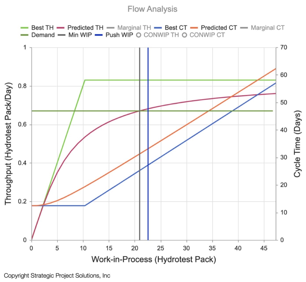
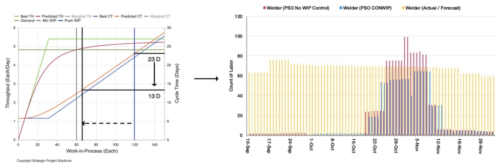
Another critical analytic is the minimum WIP required to meet the targeted demand (desired throughput rate), typically represented by schedules & quantities in construction (Figure 8). The Best Throughput curve shows the maximum throughput for a flow under zero variability and the Predicted Throughput shows the throughput that can be expected based on given demand variability and process steps variability. The greater the variability, the further away the TH and CT curves are from the best curves. This validates the comment above that capacity (TH) can be increased by reducing variability. As can be seen, the larger the amount of WIP, the greater the TH with diminishing return as WIP increases. Simultaneously, CT increases as WIP increases without limitation. Since increased CT represents the amount of time work is trapped within the flow, it can be interpreted as the minimal amount of time investment that is trapped within the flow. Increased WIP (amount) for increased cycle time (duration) is a double whammy to the economics of the investment. Therefore, determining the minimum WIP that delivers the demand is critical. Figure 8 shows minimum WIP where the Predicted TH curve crosses over the demand line.

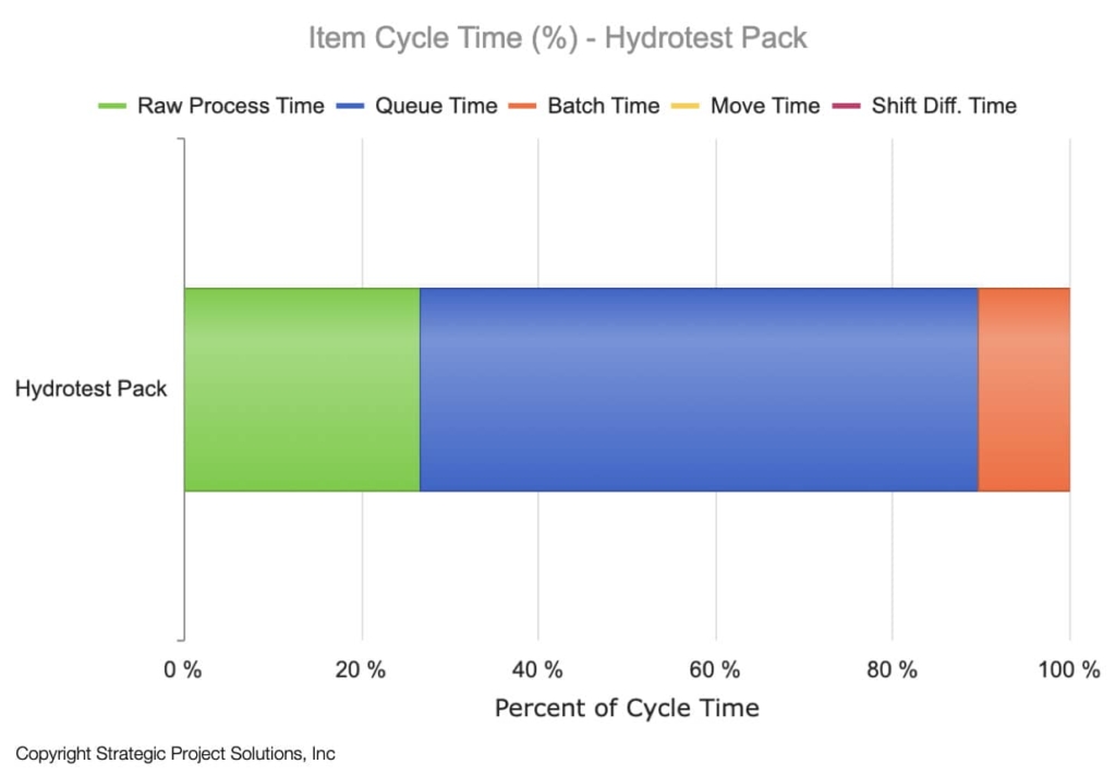
If there is a desire to further compress the cycle time in addition to ensuring that only the appropriate amount of WIP is in the system, it is important to understand what drives the current cycle time. Since the resulting cycle time is not just a function of time the work is being done (process time), but also the amount of time work is waiting due to queuing, batching, etc. (Choo and Spearman 2019), we can understand the proportions of cycle time that each component contributes to. Figure 9 shows the distribution of each component that makes up the overall cycle time. In this case, process time only makes up 27% of the overall time with queue time taking 63% and batch time taking 10%. Therefore, the initial target for optimization would be to reduce queue time. Which levers to pull to achieve this? The answer resides with the Kingman’s equation (one of the key equations in Operations Science).

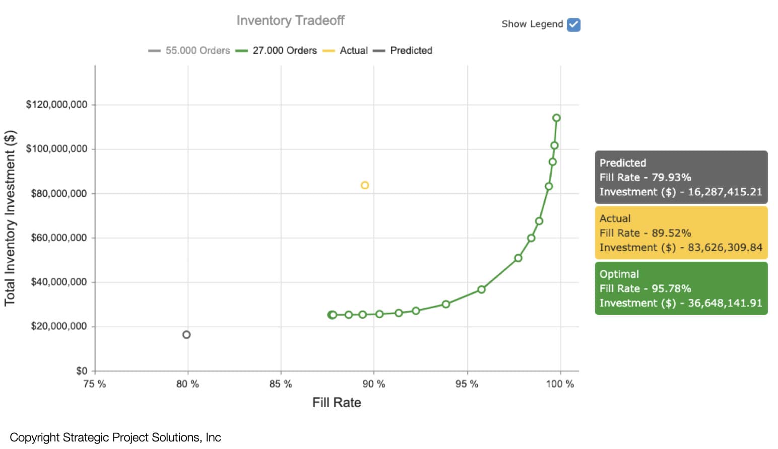
If the production system relies on large amount of raw material stocks as well as partially completed assemblies and there is desire to reduce the amount of cash tied up while improving fill rate¹, analytical modeling provides a robust and quick way to optimize stock policies such as reorder point (ROP) / reorder quantity (ROQ) across all items at once. The resulting optimization provides optimal frontier (green curve in Figure 8) that leadership can use to determine the appropriate trade-off between investment tied-up in stock vs fill rate.

[1] Fill rate is defined as the fraction of demands that are fulfilled from stock (Hopp & Spearman 2016)

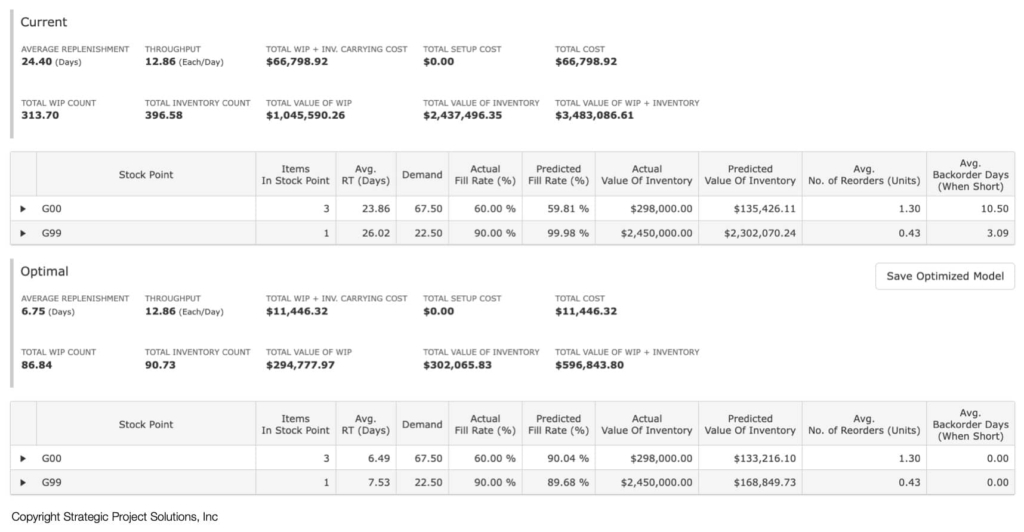
The some of the analyses and optimizations above apply to when answering questions related to making things (Figure 7, Figure 8, and Figure 9) or buying things (Figure 10). What if you are your own supplier where you are building inventory of parts, assemblies, systems, etc. so that they can be used for subsequent process? Figure 11 shows concurrent optimization of WIP and stock that allow highest possible capacity utilization (minimize cost) while meeting desired service level.

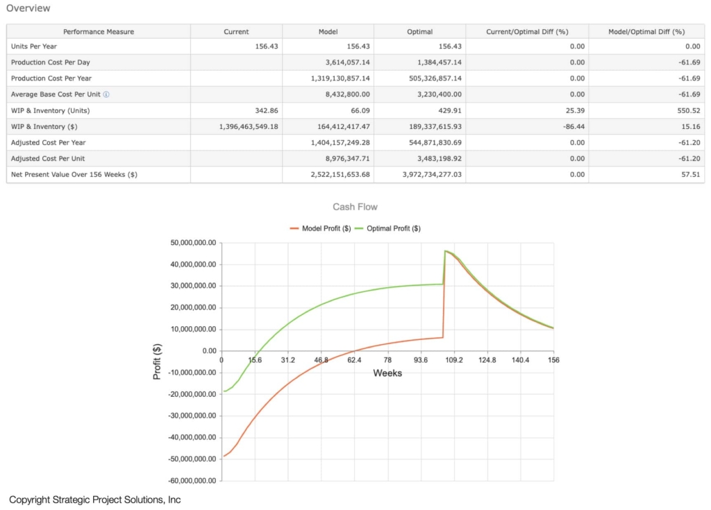
Additionally, analytical modeling can be used to determine the optimal resource profile that maximizes NPV by incorporating the revenue that would be generated, whether it be once or sustained over a period like putting oil & gas wells, solar panels, wind farms, etc. (Figure 12)

As shown above, the result from analytical modeling is highly insightful and relatively easy to get to. However, it requires the system to be in a steady state, where the variables of interest like demand, process rate, number of resources, do not change for a given period. We’ve found that in construction projects, operations related to design, engineering, fabrication, transportation, assembly, commissioning work, reach this state beyond the initial build-up phase and before final finishing phase. There are projects that are too short to achieve a steady state, or the environment keeps changing that they never reach the steady state. In these cases, DES is the best means to analyze and optimize production systems with these characteristics. To explore how to approach this, let’s take a look at DES.

Discrete Event Simulation

DES models a production system by analyzing the status of the system at the start of an event and end of an event. For example, at the start of an event, the DES engine “grabs” all the required inputs from the queue of inbound inputs in the required quantity (raw material, design/engineering information, etc.) and the resources from pools of resources (labor, equipment, space, etc.) and holds these inputs and resources for the duration of the task (deterministic or stochastic based on the distribution used), and then releases these inputs and resources at the completion of the process. The outputs then go on to the next steps and the resources go back to the pools, unless the resource is bound to the outputs, e.g., some crew may stay with a module / system / area until it has completed all the processes. Example of the process may be conceptualized as Figure 13. The demand into the production system can be determined by a rate (same as analytical model) or can be determined by the schedule assumptions (e.g., how schedule defines big batches of infrequent arrivals of material, information, etc.)

Since it is grabbing resources only when available, the maximum capacity utilization in DES models is 100%, so the consequence is that and any demand over the capacity will be absorbed by additional time. The following sections include some of the analytics that can be generated using DES models that are useful in optimizing production systems.

One of the most critical analytics valuable outputs of the DES is the total duration. Whereas analytical model assumes a steady state, the DES model can be designed to have a distinctive start and end which means total duration can be computed. If the model is stochastic and the simulation is run multiple times, the overall duration will vary resulting in a profile that resembles Figure 14.

The other analytic that is important to understand is capacity utilization over time. If WIP is not maintained at certain level to keep the utilization steady, operations will begin as soon as all the prerequisite work is completed and the resources are available. This will cause the resource utilization to fluctuate, sometimes greatly, over time (Figure 15). If there is sustained period of near 100% utilization for a resource, the operations that are performed by this resource will result in extended cycle times unless this operation is the first in the process. This will cause WIP to fluctuate as well resulting in a WIP curve shown below (Figure 16). This insight is critical when determining the maximum work area sizes required to perform the work including laydown and staging areas.

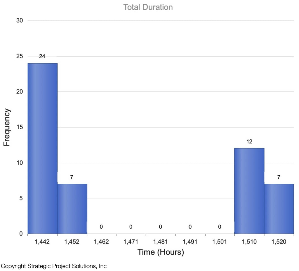
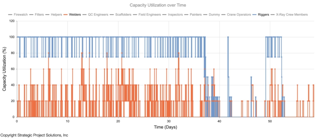
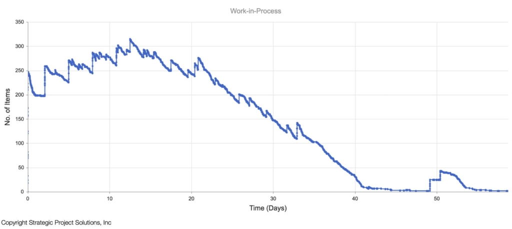
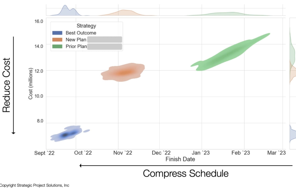
Figure 17 show the two-dimensional density plot of DES in terms of cost and schedule. As can be seen from the plot, the prior plan (original plan) shows the higher cost and longer schedule with large variability compared to the best outcome (best DES result) which has lower cost and shorter schedule with much more predictability. “New Plan” shows the predicted result of what the project team resulted to import based on the required changes. The ability to predict this outcome is critical as alternatives can be examined to see if the changes are worth making by performing series of “what-if” analysis.

Integrating Discrete Event Simulation With Analytical Modeling

To better illustrate this integration, we will use an example to examine how insights from Analytical Model can make the use of DES more effective and efficient.

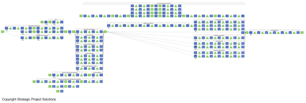
The following diagram is a production system map of jacket fabrication & assembly for an offshore drilling platform involving labor resources such as welders, riggers, and equipment resources such as cranes, forklifts, etc.

Based on the original schedule, Figure 18 shows the amount of demand (represented using man-days) that SHOULD be executed throughout the production system.

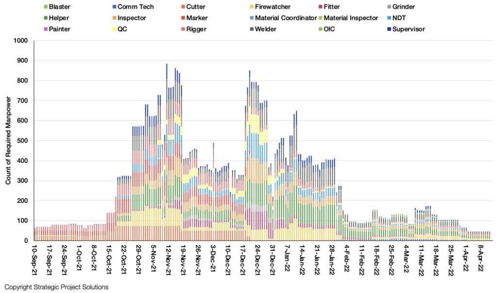
Figure 20 shows the average capacity utilization for each of the resources during the peak demand period. This quickly exposes a hidden production risk, which is that Riggers and Welders are substantially undersized to deliver the rate of work that is required to deliver the project as per the original schedule (represented by 388% and 145% utilization for Riggers and Welders respectively). Since the resource with the highest average utilization is defined as the bottleneck in Operations Science, Riggers are the bottleneck for this production system.

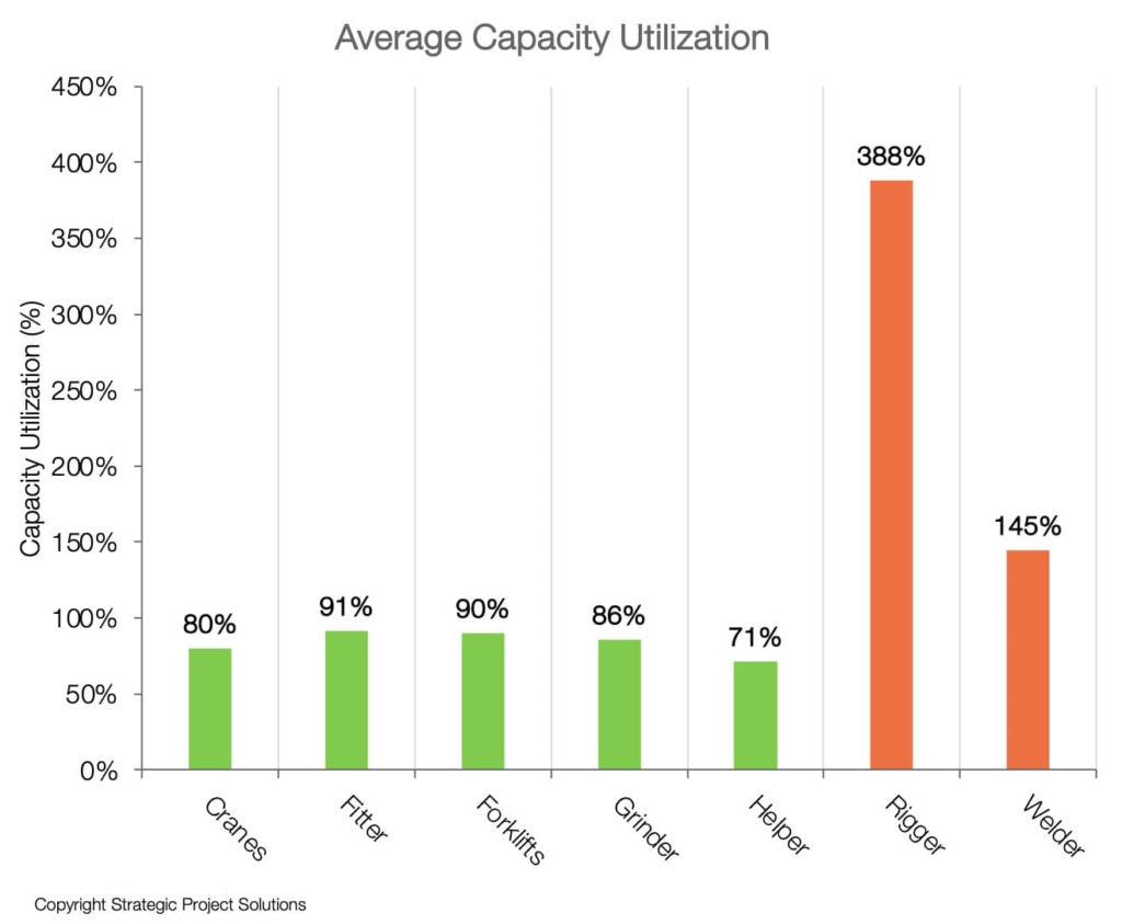
The project team indicated there is lack of specialized welders in the local market while additional riggers are easier to find, so the question was how to create more welding capacity without increasing welders, especially in peak periods per the original schedule. Figure 19 shows the comparison of welder requirements between the original plan, actual / forecast and DES model. Original plan (indicated by “Plan”) shows the original manpower loading plan.

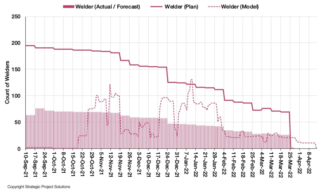
It can be seen that the plan was to have the highest number at the beginning and then start reducing the number of the welders as the work progressed. The actual/forecast shows that they could not get all the desired number of welders per the manpower loading plan and is forecasting to only have a limited number until the end of the project. But the DES exposes a very interesting insight depicted in the model curve, which is the actual requirement of welders according to the behavior of the production system, painting a very different picture. To reduce the peaks and valleys of demand for welders, while ensuring they are only working on the right work in the right sequence and minimizing the cycle time through the production system, WIP control needed to be looked at.

Figure 20 shows how Flow Analysis results from the analytical model can be used to determine optimal amount of WIP in the production system to reduce CT time, while delivering the desired TH, i.e., demand. This allows the peak of the resource requirement to be less than the amount available. With the right sequence control using Project Production Control (outside the scope of this paper but refer to Arbulu, R.J. et al. 2016), effective use of resources can be ensured.

Conclusion

Achieving predictable project schedule and cost while maintaining desired safety, scope, and quality, has been and continues to be an objective of constant pursuit by owner/operators, contractors, vendors as well as academics and solution providers. To do so, many rely on building a model that describes either what needs to happen or predict what might happen using common project management approaches.

Whether it be deterministic and stochastic, schedule-based approaches are not able to accurately model the behavior of interactions between inputs, resources and operations under variability and dependency. By appropriately integrating analytical model and discrete event simulation, robust models can be built effectively and efficiently to allow more robust, insightful and faster analysis to identify opportunities to optimize project production systems.

When applied properly, production modeling provides insights into new set of decisions for project leaders that cannot be seen using traditional approaches that sets up projects for success.

References

Arbulu, R.J. and Choo, H.J. (2020) Five Levers of Production System Optimization. PPI Technical Guide, Project Production Institute

Arbulu, R.J. et al. (2016) Contrasting Project Production Control with Project Controls. Journal of Project Production Management Vol 1., Project Production Institute

Choo, H.J. and Spearman, M.L. (2019) Cycle Time Formula Revisited. Journal of Project Production Management Vol 4., Project Production Institute

Hopp, W. J. and Spearman, M. L. (1996). Factory Physics Waveland Press Inc.

Martinez, J.C. (1996) STROBOSCOPE: State and resource based simulation of construction processes. Ph.D. Dissertation. University of Michigan

Senecal, P.K. (2020) Automated Meshing Facilitates Simulations for Optimizing Systems. Pumps & Systems. https://www.pumpsandsystems.com/improving-pump-compressor-performance-computational-fluid-dynamics

Shenoy, R. and Zabelle, T.R. (2016) New Era of Project Delivery – Project as Production System. Journal of Project Production Management Vol 1., Project Production Institute

Teicholz, P.M (1963) A Simulation Approach to the Selection of Construction Equipment. Stanford University. Department of Civil Engineering

Tommelein, I.D., and Ballard, G. (1997) Look-ahead Planning: Screening and Pulling. Technical Report No. 97-9, Construction Engineering and Management Program, Civil and Environmental Engineering Department, University of California, Berkeley

Zabelle, T.R. (2024) Built to Fail: Why Construction Projects Take So Long, Cost Too Much, And How to Fix It. Forbes Books