Capital project owners and service providers may be blind to the fact that working with excessive amounts of inventory contributes to longer schedules, cost overruns and impact to cash flow, which negatively affects return on investment. On the other hand, not enough inventory and the project will not achieve the required throughput while also compromising cost and schedule targets. So, in the spectrum of too much and too little, is there an optimal point? What are the drivers of this optimal point? Can we determine it, and if so, how?
This paper demystifies the common belief that running projects with high levels of inventory represents best practice without negative consequences and explores why we should be concerned about it. It does this by examining what inventory means in the delivery of capital projects, what its components are, and how optimal values can be determined using Operations Science as the technical framework. The paper examines several project examples and concludes with recommendations for how to consider the impact of inventory when making decisions across the project lifecycle.
Keywords: Inventory, Operations Science, Production Systems, Stocks, Work-in-Process.

Roberto Arbulu is Senior Vice President of Technical Services for Strategic Project Solutions. He has more than twenty years of experience in the delivery and optimization of energy, industrial, technology, and infrastructure capital projects and has worked with numerous owner operators and service providers across North America, South America, Europ ...
Contrary to common belief, inventory is not well understood in the world of capital project delivery, much less its impact to project performance. When project professionals talk about inventory, they typically refer to certain amount of materials needed to support onsite construction; in other words, ‘stocks’ of materials including permanent equipment. This should not surprise us because the terms inventory and stock are considered synonymous, so people use them interchangeably all the time. Even in Operations Management literature, most inventory policies mean stock policies.
However, from a production perspective, inventory and stock have different meanings altogether. In fact, inventory includes more than just stocks of materials. Attempting to discuss the implications of excessive (or not enough) inventory without exploring the production view of inventory will result in a myopic perspective. As the first piece of the puzzle, this paper elaborates on basic definitions and differences between these terms to set a foundation for a more robust discussion.
With clear definitions, the second piece of the puzzle explores common project delivery practices behind how project teams make decisions about inventory including the thinking (or lack of) that drives these practices. The third piece of the puzzle proposes a method that uses the science of operations to determine what level of inventory is optimal. In both cases, we are referring to inventory across the end-to-end project production system including how we design, engineer, fabricate, assemble, transport, install and commission assets.
By ‘production view,’ we mean understanding inventory and the role it plays in a project production system and its performance over time. As such, we will adopt Operations Science ([1],[2],[3],[4]) as the technical framework to understand what inventory means when producing across the project delivery lifecycle and break it down to its components.
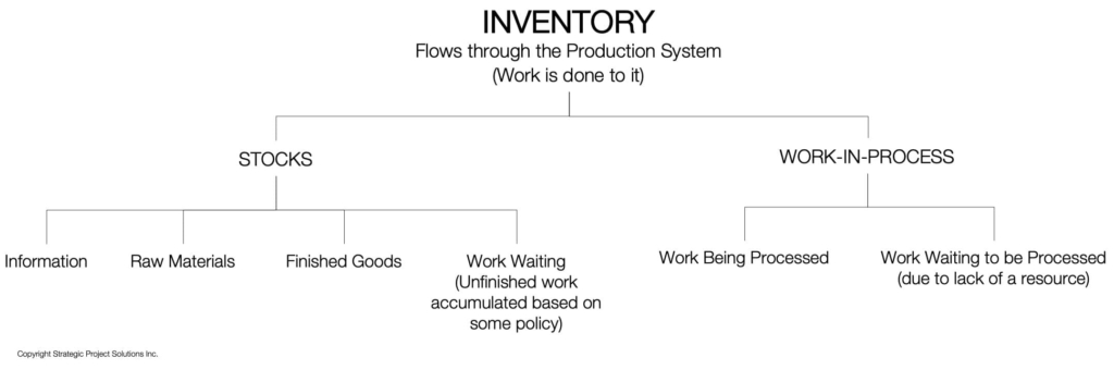
Operations Science sets forth that inventory in any production system, including those of projects, has two components, stocks and work-in-process (WIP), resulting in the following frame:
Inventory = Work-in-Process* + Stocks
* Be cautious here as work-in-process is not the same as work-in-progress, even though they use the same acronym. Work-in-progress is a measurement used in Earned Value Management (EVA) and typically expressed as a percentage.
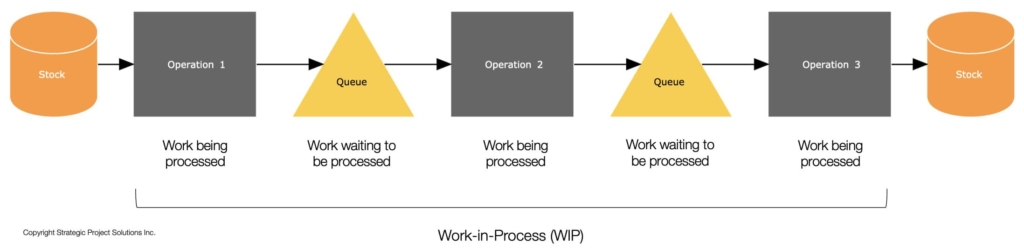
This simple relationship will assist us to explore later what excessive inventory really means. As stated previously, the global engineering and construction industry is familiar with the concept of stocks, but unfortunately, it is not fully familiar with the concept of work-in-process. Work-in-process is a key measurement of the health of a project production system and its ability to effectively respond to certain demand. Work-in-process represents a quantifiable number of units of work (e.g., number of piles, number of engineering deliverables, etc.) that 1) are either being processed at any given time by one or more operations in a production process, and 2) are waiting to be processed in between certain operations in a production process (waiting on queues due to lack of a resource). We can therefore understand WIP as the following:
Work-in-Process = Work Being Processed + Work Waiting to be Processed
To illustrate the above frame, refer to the following schematic that includes three sequential operations depicted using rectangular boxes and two queues depicted by triangles. Depending on how work gets transferred from one operation to another, the readiness of resources in a subsequent operation to take on work that arrives, and the variability of executing the work itself, queues of unfinished work will be formed in between operations and across the production process. In simple terms, WIP is the count of the number of items in all the boxes plus the number of items in all the triangles at any given time during production.
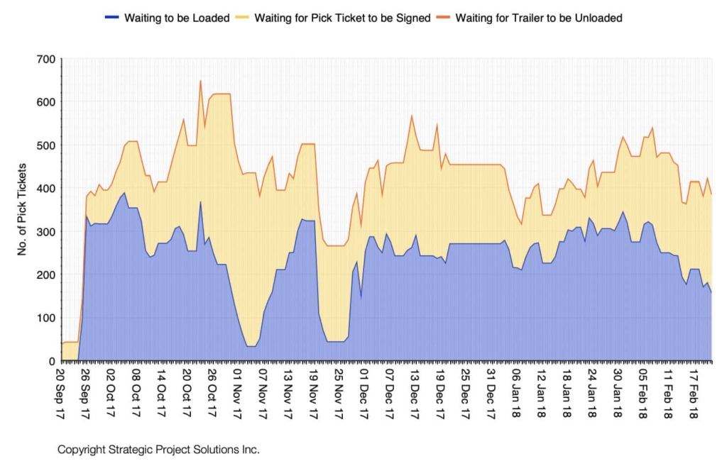
Because project production processes typically remain active for multiple days, weeks or even months, measurements of ‘actual’ WIP levels will vary over time, meaning WIP today may not be the same as WIP tomorrow or the same as yesterday or a week ago (unless CONWIP1 is used). In practical terms, if you select a project production process of choice and plot actual WIP levels over time, you will end up generating a curve as illustrated in the next example.
[1] CONWIP stands for Constant Work-In-Process, and it is a production control protocol designed to maintain a constant level of WIP in production systems.
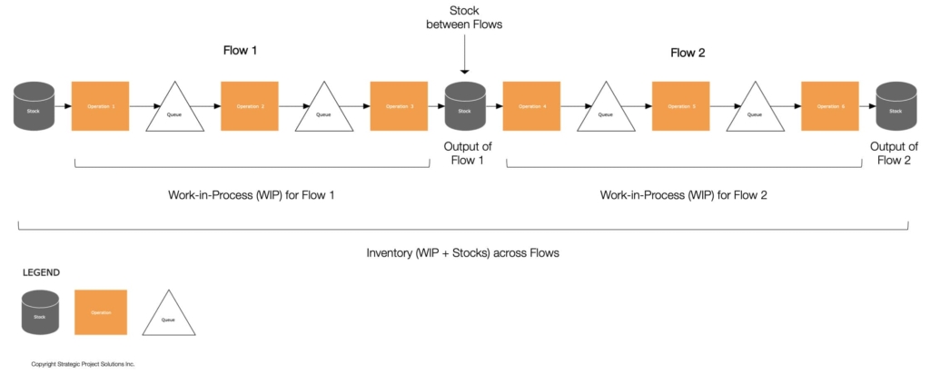
To complete the production perspective of inventory, we need to add stocks to the picture. Stocks refer to a set of certain items, which may include, for instance, raw materials as inputs to an operation, or goods that are outputs of a production flow (e.g., finished goods, assemblies, engineering packages, etc.). To illustrate this graphically, refer to the following schematic of a generic production system map, which incorporates WIP as well, where one production flow (Flow 2) operates based on outputs of another production flow (Flow 1), both part of the same production system, and where stocks are represented by cylinders.
What this means is that when analyzing production systems, we cannot and should not use inventory and stocks as synonymous because we will be missing the second element of inventory: WIP. A discussion about excessive inventory must therefore include WIP, not just stocks.
Furthermore, it is important to highlight that people may think about production in projects in physical terms, meaning craft-based production as when we fabricate, assemble, install and commission things. Although this perspective is not wrong, we may be missing the fact that production can also be non-physical as when we design and engineer the systems in an asset. The point is that the concept of inventory includes non-physical and physical production across project production systems, consequently, stocks and WIP can represent non-physical (e.g., information) and physical (e.g., materials, assemblies, finished goods) items.
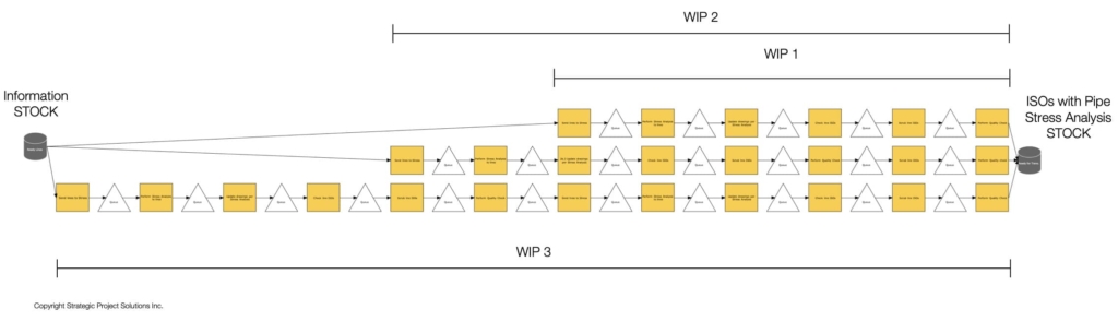
For illustration purposes, the example below depicts a non-physical production system that produces isometric drawings (ISOs), in which pipelines go through three alternative production processes to conduct stress analysis on the pipe. Therefore, each of the three production processes contains its own WIP levels, while using the same stock of information (stock on the left) and generating ISOs with pipe stress tests (the output stock on the right).
The definition of inventory by the Project Production Institute (PPI) [2] summarizes it well:
“The accumulation of entities that occurs anywhere within and/or between processes (flows) is called Inventory. Inventory between two or more flows is called stock, while inventory within a flow is called work-in-process or WIP.”
To expand on this, the following classification provides stock types and elements of WIP, all part of inventory.
Now that we have defined inventory as stocks plus work-in-process, the question is how the global engineering and construction industry approaches how much of what to have where, when and for how long, and how much to be producing at any given time. It is not the intent of this section to conduct an exhaustive analysis of all current practices, but rather explore the most common ones based on the author’s experience and differentiating practices related to stocks and WIP [8].
When it comes to the stocks side of inventory, the most common practice in the industry is to plan and secure access to as much space as possible as in dedicated onsite laydown areas and warehouses to keep as much as possible of as many materials as possible as early as possible according to how project progresses. People prefer to be looking at things than looking for things. Also, the thinking here is that as the cost of materials is included in project budgets and we plan to use them anyway, why not keep them on site.
When access to space on sites is very limited, project teams are forced to rethink these practices to match stock sizes to the available space (e.g., building construction in metropolitan areas, offshore oil platforms, etc.). However, even in these cases, this does not mean those stock sizes are optimal sizes. Despite space limitations on site, others opt to secure access to nearby facilities to act as warehouses for the volume of stocks arriving to site. It is not uncommon to see offsite warehouses in addition to onsite warehouses. The larger the project, the more we see the situation escalating to massive volumes as illustrated next.
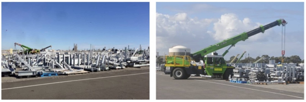
The unintended consequences associated with this type of practice are several [7]. For instance, the time required to amass the stocks (accumulate into a mass), the cost of the resources needed to handle the stocks including equipment and labor (e.g., move things around, etc.), the cost of the infrastructure itself as it may not be free, and even if free, the cost of preparing it to hold the stocks, the cost of establishing a full-time team to manage laydown / warehousing operations, the risk of physical damage forcing to replace materials for new ones, the risk of materials becoming obsolete as design changes may occur when stocks are already waiting somewhere in the chain, the risk of physical degradation over time making materials not fit for use, the need to preserve permanent equipment while it waits on stocks, the risk of theft, not meaning stolen by thieves, but materials assigned to one team being used by another team, and the cost of surplus because we order more just in case. And perhaps the most important of all, the amount of cash tied up in those stocks (access to cash is not free). What all this means is that the price is not the cost. What we pay for an item is not what it costs us to have it ready to install. This increases project final cost (and time as well) as this hidden cost is not contemplated in anybody’s budget.
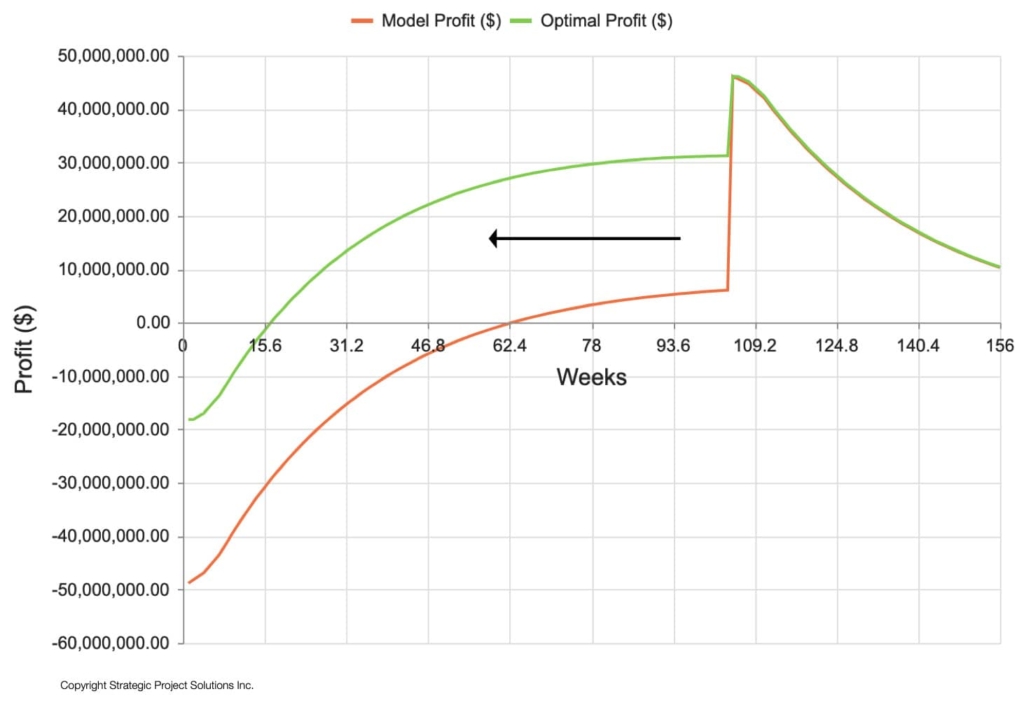
Inventory (stocks and WIP) has a direct impact on cashflow (inventory created during the project delivery process is all cash outlay). The amount of cash outlay prior to recognizing revenue is a fundamental element in calculating net-present-value (NPV) and return on invested capital (ROIC). The less cash needed, the better the financial return. Therefore, managing inventory is the same as managing cash. Using too much cash / inventory impedes pursuit of other project opportunities including the ability to invest in additional projects. The following chart illustrates the impact of operating based on optimal inventory levels to cash flow (moving the curve from a current state model not optimizing inventory to the left).
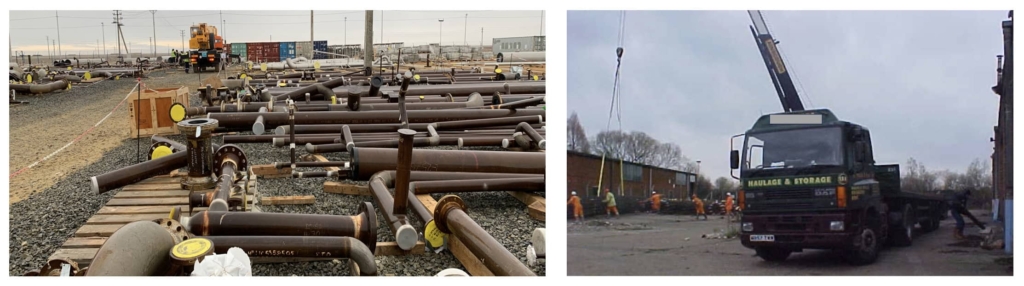
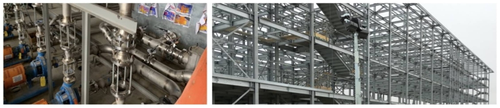
The above applies to all types of materials and permanent equipment, meaning made-to-stock, made-to-order and engineering-to-order (including configured-to-order). However, these practices have an additional effect in the case of engineered-to-order items such as pipe spools, pumps, skids, modules, etc., as items are not interchangeable (e.g., a pipe spool goes into a specific location), and sequence comes into place. Basically, we can have a large stock but if we don't have the right item to follow a desired installation sequence, we are forced to install other items as we wait for the right one, creating more open workfronts (more WIP). The following photos illustrate this situation, where dedicated cranes and crews are looking for the right items in the sequence (the right spool on the left photo) and offloading excessive materials (rebar pile cages on the right photo), where double handling, quality and health and safety risks are evident.
Behind this way of thinking and doing is a strong emphasis on keeping labor busy as much as possible ensuring they don't stop working because of lack of materials. It is also influenced by optimizing the means of transport based on full loads, while in many cases, multiple loads are scheduled for delivery at once. Furthermore, percent complete accounting does not recognize excessive inventory, but rather makes the focus on saving labor cost. Under this conventional construct, labor becomes the presume only variable to play with.
Contrary to the idea of stocks, the engineering and construction industry does not understand work-in-process nor systematically apply fit-for-purpose methods to dimension and control WIP on projects. However, people allude to it using other expressions such as the number of workfronts or work packages being executed in construction, number of items being fabricated or assembled this week, number of workstreams or deliverables an engineering team is working on, to name a few. Other expressions like ‘it is completed, but not done’ exemplify what typically occurs when doing work resulting in progress gained through Earned Value, while work is still to be done onsite. One of the reasons why S-curves reach +90% progress while completing the last 10% takes a lot of time, and in many cases burning “non-progressable” hours.
The examples below illustrate how WIP physically manifests on construction sites. On the left, multiple valves are missing, but to install / align the pipes and account for them in progress reports, special threaded rods have been fabricated to precise measurements and then installed, which is not free. When the valves arrive, labor needs to be used to remove the rods, disassemble the connections and realign. The other example shows the complete steel structure of an entire 4-story building; however, no other type of work has started (e.g., slabs, façade, etc.), other than the crew installing the steel staircases. This translates into a large WIP of steel components waiting for the next wave of work. If by design, the project team decided to complete the entire steel structure as shown and then let other work start, that picture would be represented as a stock of unfinished work in a map of the building production system. Additionally, in this case, a large stock of fabricated steel components was needed to build the whole structure.
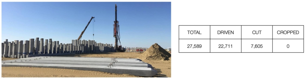
This next example looks at a pre-cast piling production system, where the total number of piles to be installed is 27,589, while the piling installation production process has three main operations: 1) drive the pile to certain depth, 2) cut part of the pile left above ground, and 3) crop the top of the pile to expose the rebar to connect to the foundations.
At a specific point in time during site execution, the project team reported the data in the following table. This data indicates that 82% of all piles are already driven into the ground, and 27% already cut, but nothing cropped yet. In other words, the throughput of the piling production system is zero, which means work is not being released to the next trade to do work (e.g., crews working on foundations).
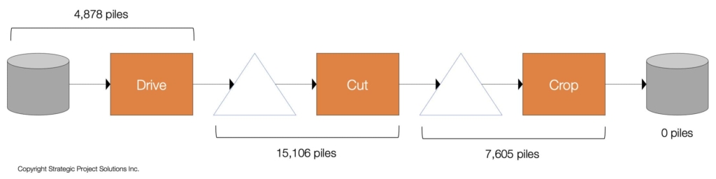
To better understand how this system is behaving, we should visualize the production process including operations and queues as shown next. As 7,605 piles have been already cut, we can conclude that some are at the queue between Cut and Crop and some are probably being cropped, but the data does not allow us to establish exactly how many are at the queue or being cropped. Since 22,711 piles are already driven and 7,605 already cut, we can conclude that 15,106 are waiting to be cut and being cut, but again, the data does not allow us to differentiate how many are in the queue vs. the operation. With all this work in the system (15,106 + 7,605 piles), we can also conclude that there are 4,878 piles either in the initial stock of piles entering the system or being driven. What is certain in this case is the fact that at least 22,711 piles are in WIP, while not a single pile has yet made it through the entire production system. Someone designed this production process to optimize the productivity of the pile drivers (e.g., typically Drive earns more progress than Cut and Crop), but not to optimize the throughput of the entire system of completed piles ready for foundations. While the S-Curve may have shown ‘good’ progress, the production system was not releasing work to the foundations production system that follows. This is because the cycle time per pile increased due to the high WIP of piles. Examples like this abound in construction. It is a matter of looking closely and doing it from a production perspective to understand how systems behave.
The accumulation of unnecessary WIP in project production systems is driven by a strong emphasis on gaining progress and improving the productivity of labor and construction equipment. The industry cares more about capacity not waiting for work than work waiting for capacity (part of WIP). Why is this important? Identifying optimal WIP levels and controlling WIP is, in fact, much more relevant to increase production system throughput than increasing productivity at each individual operation resulting in faster schedules, less cost, and better return on capital investment.
The title of this paper refers to excessive inventory, which implies something is beyond certain level. And if something is beyond certain optimal level, there should be implications of operating beyond that optimal point. A simple real-life example (not from projects) is the measurement of human body temperature. We know the normal temperature should be in the range of 97 F to 99 F for adults, and 95.9 F to 99.5 F for children, so if the human body operates exceeding the normal threshold, high fever causes system malfunctioning, and if not properly controlled, this can result in death. Similarly, if the human body operates below normal temperature levels, severe hypothermia also causes system malfunctioning leading to rapid death if actions are not taken.
When it comes to inventory, it works the same way. Through Operations Science, we can calculate optimal levels of both stocks and WIP in any project production system responding to certain demand. We will call ‘excessive’ to any actual amounts beyond the optimal levels and not enough to levels below. In either case, there are consequences. Operating with less-than-optimal levels will starve the system not allowing it to meet demand, and more than optimal only increases time and cost.
The following are two different examples of how project teams identified optimal levels of inventory (stocks and WIP) in construction production systems through an operations science approach.
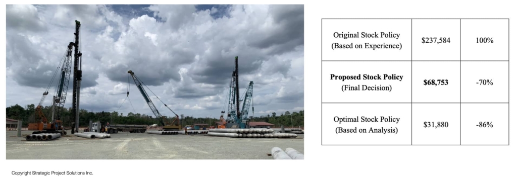
This is the case of a fuel terminal that included storage tanks, a jetty for loading and offloading product, and connecting piping. The design included the use of precast piles (jointed and pencil piles) for the jetty and other project areas. A jointed pile combines a top pile with a pencil pile where the top pile seats on top of a driven pencil pile, it is welded in place, then driven further into the soil. While the piles themselves were standard designs, they were made to order for the project. The project team was interested in determining opportunities to optimize the supply of these two types of piles (top and pencil) including identifying optimal levels of stocks on site without compromising the planned construction sequence. This section focuses on how they analyzed optimal on-site stock levels and compared them with what they originally thought they should have based on experience.
Knowing that schedules set the demand for project production systems (demand = expected throughput rate), the first step was to understand what demand was being imposed onto the production system [6]. Combining the use of the schedule and bill of quantities, a demand profile for top and pencil piles was produced indicating that at peak the project needs 14 top piles per day and 18 pencil piles per day, while average weekly demand was 78 top piles and 87 pencil piles.
The team generated a production system map for the piles including fabrication, delivery and site installation as illustrated below and targeted to find not only optimal onsite stock levels for top and pencil piles, but also reordering points and reordering quantities based on demand, supply capacity and replenishment time. The selected pile supplier was located less than an hour drive from the project site and had capacity to produce 30 precast piles per day. Fabrication included 2 weeks to allow the concrete to cure and strengthen as a requirement for transport to site. Historical data indicated that the installation rate for pencil and jointed piles was 8 and 5 per rig per day respectively.
Using the map, production system and inventory models were created including parameters such as lead times, variability in demand and supply, demand and supply rates, to name a few.
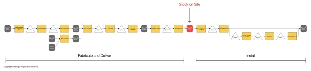
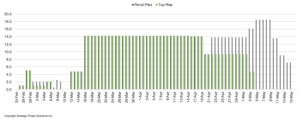
When analyzing optimal onsite stock levels (red cylinder above), a Stock Trade off curve was generated to graphically depict the exponential trade-offs between targeting a given fill rate and the cash tied up in the stock. In this case, the chart shows three curves, each representing different replenishment policies for both pencil and top piles. Each replenishment policy had a distinct effect on the total stock investment (cash tied up in pile stock) and fill rate (the percent of demand that is met from the stock). In essence, if a high fill rate is desired, the effect is more stock on hand, and therefore, more cash tied up in stock. All points in a curve are considered optimal for a desired fill rate.
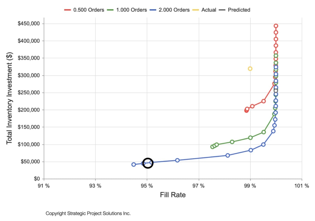
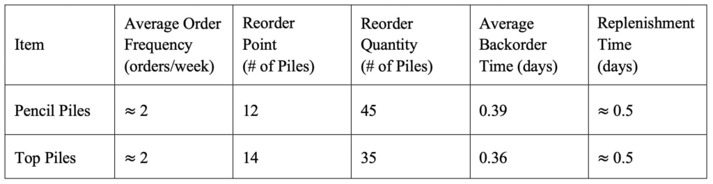
The red, green and blue curves corresponded to different order frequencies: 0.5, 1, and 2 orders per week. It was clear from the plot that an order frequency of 01 order every 2 weeks (0.5 order per week) would force the project to hold on to more stock than the other order frequencies. Given the fabrication facility was an hour away from site, considering the supplier holds some minimum stock level of finished goods (piles ready for transport) making backorder time short, and the limited storage space on site, a fill rate of 95% was selected for an order frequency of 2 orders per week. These policies established the reorder points for pencil and top piles to be 12 and 14 respectively and the reorder quantities for pencil and top piles as 45 and 35 respectively. When stock levels for each pile type reach the reordering point, an order is placed equivalent to the reordering quantity for each pile type. No orders are placed for additional piles unless stock levels have reached the reordering point. The following table and charts summarize the optimal replenishment policies as well as stock profiles and associated cash tied up over time.
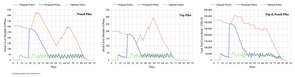
Prior to this analysis, the team established a desired stock policy based on their experience, which was included into the analysis for comparison purposes. These appear in the above charts as original policy. In average, the original stock policy required a stock of top and pencil piles on site equivalent to USD $237,584, while the optimal policy reduced the cash tied up to USD $31,880, meaning 86% less stock without compromising installation rates. The project team opted to almost double the optimal stock policy to USD $68K to be on the safe side, however, even doing this represented a reduction of 70% from the original policy.
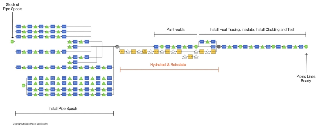
This is the case of the construction of an industrial plant that included a significant amount of piping of different diameters and materials. After pipe spools were fabricated, assembled and delivered to site, they would be installed in a specific sequence to form pipelines that go through producing units at the facility. Each line was broken into several hydrotest packages to ensure installed piping conforms with desired standards. To conduct a hydrotest, some elements of the pipe system need to be removed and then reinstated after the test. If the test passed, other works such as heat tracing, insulation, cladding installation and final testing followed. Although the team conducted a more comprehensive analysis of this overall production system as shown in the map below, this section of the paper focuses only on the hydrotesting and reinstatement portion of the production system to illustrate how optimal WIP levels were determined (orange section below).
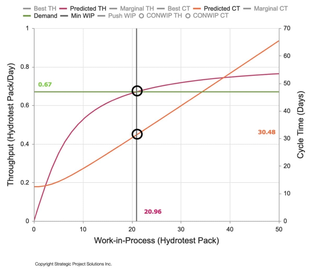
The demand imposed by the schedule indicated that the production system must have an average throughput of 02 hydrotests including reinstatement every 3 days, in other words, 0.67 reinstated hydrotest packs per day. If the production system was not able to meet the demand, the project would experience schedule delays. So, the question was asked, if the production system has the capacity to respond to the demand, what should the optimal amount of hydrotests in WIP be without compromising meeting the demand?
Production system models require multiple input parameters including demand rates, production rates, variability levels (demand and process), batching policies, types of capacity contributors and quantities, to name a few. The production system model generated a Flow Analysis Chart (shown below) that showed the relationship between throughput (TH), work-in-process (WIP), and cycle time (CT) for hydrotesting including reinstatement. The horizontal green line depicted the demand the system must be able to respond to (0.67 reinstated packs / day). The magenta curve showed the relationship between TH and WIP, while the red curve between CT and WIP, both including the impact of variability.
The intersection of the demand line and the TH curve defined the minimum WIP that the production system should have to meet demand. In this case, 21 hydrotests must be in the works at any given time. If WIP is lower, the demand would not be met (lower than 0.67 packs / day), and if the WIP is higher than 21 packs / day, TH can be slightly increased (e.g., get to 0.7-0.75 packs / day), however, the price to pay here was that the average cycle time to complete each pack including reinstatement would rapidly increase beyond the optimal of 30.5 days. For instance, if WIP was around 35-40 packs (60 to 90% more than the minimum WIP), cycle time would almost double getting close to 60 days per pack. But selecting the minimum WIP as optimal may be risky as variability in execution can increase and because of that TH can be lowered to less than 0.67 packs / day. A more prudent decision was to set an optimal WIP level to ~25 packs.
Although this example focused on an installation production system, the same type of analysis can be performed to any other type of production system including engineering, fabrication, assembly and /or commissioning, and in so doing, not only determine optimal WIP levels, but also check if the system has the capacity to meet the demand and analyze the utilization of capacity across resources including identifying bottlenecks.
This paper has established a clear differentiation between inventory, stocks and work-in-process for project production systems using Operations Science as the technical framework. It presents a significant opportunity for the global engineering and construction industry to avoid the negative impact of operating with excessive inventory levels (stocks and WIP) by determining what optimal levels should be to meet demand along with reducing the unnecessary use of cash. As illustrated, it is not uncommon for project teams adopting a production system approach to experience gains that include operating with much less inventory (WIP and stocks) reducing the amount of cash tied up, compressing schedules (by achieving shorter cycle times with less WIP), and reducing project cost.
To take advantage of these opportunities, it is recommended project teams map, model, analyze and optimize their project production systems as early as possible in the project lifecycle (before they become active for a given project) to determine optimal levels of stocks and WIP as well as other production parameters such as capacity. Furthermore, this can be done focusing on key production systems based on complexity and criticality, or selecting those that are large contributors to project cost and/or risk. But identifying optimal levels is the first step as effective means of control of WIP and stock levels must be in place, otherwise, these will grow to undesirable levels resulting in more time and higher costs.