During the past few years, oil and gas executives have begun to profess they use a “factory” or “manufacturing” approach to field development. Terminology such as “factory” or “manufacturing” is intended to connote a sense of improved operational efficiency, compared with what was achieved with previous approaches to field development.
What is meant by a “factory” or “manufacturing” approach? How does it relate to the true definition of the terms? Do these approaches actually achieve the promised gains in practice?
This paper explores what defines factory manufacturing, what makes factory manufacturing efficient and how that efficiency can be successfully applied to oil and gas field development. We show that it is misleading to draw a direct analogy between operations in field development and the production processes in a traditional manufacturing or factory environment, such as on a car assembly line. Operations Science, the science of processes for different forms of production, is the scientific framework underpinning traditional manufacturing in factories, and better approaches to field development. We use the Operations Science framework to compare and contrast the differences in “manufacturing production” that occur in field development with more traditional forms of manufacturing. We conclude with an analysis of public data showing the most effective means to improve operational efficiency in field development.
During the past few years, oil and gas executives have begun to profess use of a “factory” or “manufacturing” approach to field development both onshore and offshore. See, for example,
(Blackmon, 2019), “ExxonMobil, Chevron Are Converting The Permian Into A Manufacturing Operation.” David Blackmon, Forbes, March 2019
and
(Blum, 2019) “In a factory-drilling operation you do the same thing many times, and quickly you learn better ways to do things.” Mike Wirth, Chevron Houston Chronicle, March 12, 2019
However, not all factories are the same. And in reality, oil and gas fields are neither factories nor manufacturing facilities. In a factory, it is the parts that flow through processes. In an oil & gas field, it is the processes (e.g., drilling, completion) that flow past the parts (i.e., the wells themselves). While the “flows” in the two examples are similar, they are not identical.
Nonetheless, oil and gas field development does share many characteristics of a “batch flow” manufacturing operation. Such operations benefit greatly from the application of Operations Science, the underlying framework that is used to understand and influence all forms of production including manufacturing, service operations and projects.
In this article, we start by examining manufacturing as described in popular media and literature, such as business and industry magazines as well as general news. Manufacturing, as popularly imagined to be something like a car assembly line, is suited to making products in high volumes and with limited customization of individual products. We use this observation to introduce the idea of the Product-Process Matrix: deciding which process should be used to fabricate a product depending upon what volumes are required and what degree of customization of individual products is needed. The Product-Process Matrix is a concept unifying traditional car assembly manufacturing and onshore field development as requiring different types of processes because there are different volumes (millions in the case of cars, hundreds in the case of oil wells) and different degrees of customization.
We next proceed to give a brief history of some key historical developments in factory manufacturing, which motivated and led to the development of Operations Science. We then give a brief synopsis of the governing laws of Operations Science, which can be viewed as the science of understanding all the different processes used in the production of physical goods and services, not simply factory manufacturing. As a special case, we briefly recap how the underlying principles of the Toyota Production System follow the governing laws of Operations Science. Finally, we analyze some available data of different operators working in the Bakken field, comparing the superior results achieved by one operator implementing an Operations Science-based approach to the results of others. The superior results achieved, obtained by applying the quantitative guidance from Operations Science, lie in sharp contrast with other approaches, which draw qualitative analogies between factory manufacturing and onshore field development, but do not offer any quantitative practical guidance on how to improve onshore field development performance.
In a March 2019 article, Forbes writer David Blackmon defines manufacturing as follows:
A true manufacturing environment is one that is highly-predictable, consistently repeatable, requires known raw materials (i.e., sand, pumps and frac water), deploys specific infrastructure, and involves the disposition of waste materials.
– David Blackmon, Forbes, March 2019
However, onshore field development, while having some superficial similarities to high volume machine paced and worker paced lines, also has some fundamental differences. Both are similar in that something is being produced. In the case of onshore field development, what is being produced is hydrocarbon-producing wells tied up to infrastructure. However, in a high-volume machine paced line, like in-car assembly, typically each car is worked on individually. In contrast, today, pad-drilling implies that wells are drilled in batches, and then completed in batches, comparable to baking a batch of cookies in an oven, rather than baking each cookie individually. Such differences, as it turns out, can have significant effects on key measurements of operations efficiency, such as the utilization of a particular resource – clearly, batch operation vs individual operation use the capacity of a resource very differently.
Academics and practitioners in other industry sectors have reflected on questions such as which types of processes are best matched to different types of production, and over the last half-century, their understanding has been codified in the Product-Process Matrix, as shown in Figure 1.
Figure 1 represents the Product-Process Matrix, a term first coined in (Hayes & Wheelwright, Link Manufacturing Process and Product Life Cycles, 1979) (Hayes & Wheelwright, The Dynamics of Product-Process Lifecycles, 1979) by Hayes and Wheelwright, which examines the types of processes that are suited to fabricating products, when products are categorized according to the degree of customization and volume of production. In Figure 1, high volume, very standard products are on the right-hand side of the horizontal axis. At the other extreme are highly customized, low-volume products. Unique, bespoke, one-off products are seen on the left-hand side of the horizontal axis. A critical observation made by Hayes and Wheelwright, and subsequently elaborated and developed in operations texts such as (Schmenner, 1990), is that different types of processes are suited to fabricating different types of products depending upon their degree of customization and volume. These are shown along the diagonal of Figure 1: Job shop; batch flow; line flow (worker paced); line flow (machine paced); continuous.
Onshore field development, unlike high volume machine paced and worker paced lines, is a batch flow process (see Figure 1 below) where the “part” is a well and the “batch” is a pad and the “process centers” are the resources used such as drilling, pad construction, completion, etc. Although the system may be defined in these terms, there does not exist a physical assembly line.
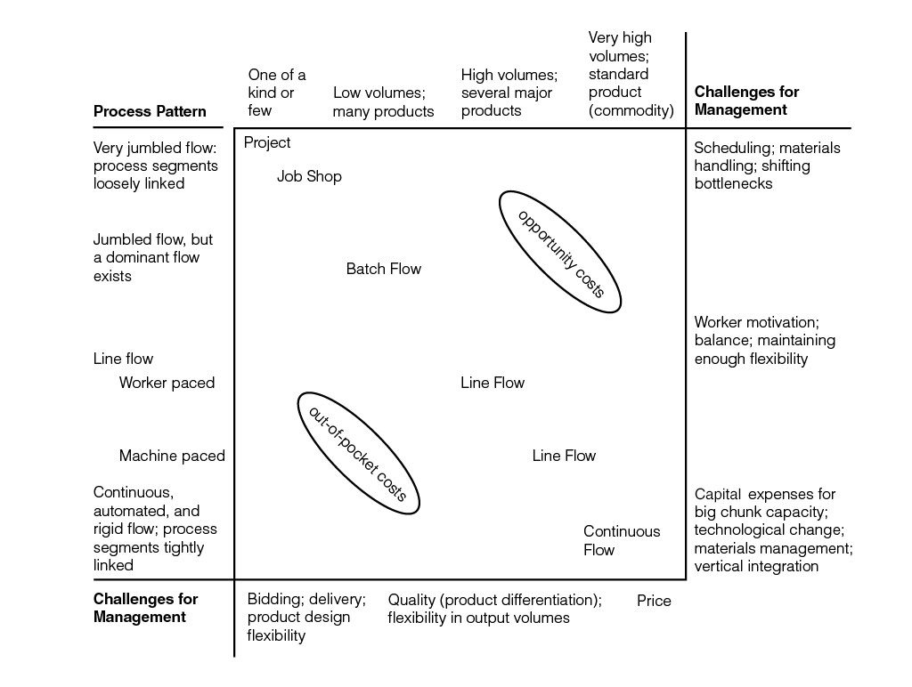
Figure 1: The Product-Process Matrix
Understanding that the production processes to make wells are not precisely analogous to a car assembly line is informative, but does not really guide the practitioner on how to configure processes in onshore field development to optimize business objectives such as how to produce the maximum number of hydrocarbon producing wells while consuming the least amount of cash in the field development process. In this section, we describe some of the considerations that occurred in manufacturing systems to motivate our description of the Operations Science framework. This unifies the treatment of the manufacturing assembly lines that is typically evoked by the term “factory approach” with a useful analytical approach to oilfield development operations.
The numbers of wells produced in oil field development (e.g., 100 wells per year) is extremely small compared to the moving assembly lines found in many automobile factories (e.g., over 100,000 per year), or even worker paced lines (e.g., over 10,000 per year). And even if field development could be managed like a high-volume factory, as Western automotive manufactures learned, not all high-volume manufacture systems are equal.
In the early 20th century, Henry Ford developed the moving assembly line to achieve high volume/low-cost production of cars. To facilitate this, Ford offered a very limited selection of vehicles – the Model T was produced for 19 years before Ford switched to the Model A and “you can get any color you want as long as it is black.”
In 1908, William Durant began consolidating his own Buick Motor Company with the Cadillac, Oldsmobile and other automotive companies to form General Motors and begin a path away from Ford’s single model strategy. This move was completed later, when Alfred P. Sloan reorganized GM and set as his goal “a car for every purse and purpose.” This strategy was stunningly effective, and GM increased its market share from 12 percent in 1921 to 32 percent in 1929 and to 47.5 percent by 1940. To achieve this, GM would make long runs of a given model before changing over to another model. This made GM very efficient in terms of unit cost but continued to limit the number of options available to the customer.
After the Second World War, Japan’s economy was in shambles. At Toyota Motor Company, Taiichi Ohno, long an admirer of Henry Ford, realized that Toyota could not adopt the successful GM strategy of mass-producing fewer types of cars. He began a journey that took Toyota from a company known for its inexpensive cars to the company who produced the Lexus luxury car.[1] One of the ways Ohno accomplished this feat was to reduce setup times from more than an hour to less than 10 minutes. Another way to control work in process (WIP) using what he termed, “just-in-time” production. Finally, he sought to remove all defects by stopping the assembly line whenever there was a problem and solving the problem right then. These methods make up the essence of what is now known as the “Toyota Production System,” a strategy that has been imitated by many American companies.
Japan and Toyota were ignored by most in the US until the Oil Crisis of 1973 when small cars quickly became more popular. Suddenly, it appeared that Toyota had advanced well beyond both Ford and GM and academic researchers began to explore how this happened. Soon, a plethora of publications including Japanese Manufacturing Techniques, (1982) by Richard Schonberger, Zero Inventories, (1983) by Robert Hall, and later The Machine that Changed the World (1990) by James Womack and Daniel Jones introduced the world to the techniques of Toyota’s approach to high volume manufacturing.
Unfortunately, none of these texts provided an adequate explanation of how TPS worked. Schonberger suggested three principles: small lot sizes, total quality control, total preventive maintenance. Hall suggested that “pull production” was the answer but never gave an adequate definition of “pull.” Womack and Jones recommended that we “eliminate muda,” the Japanese word for waste. But it turns out that “waste” is hard to define, although there were attempts (e.g., Womack and Jones, “any activity that consumes resources but creates no value to the customer”). This led to a long debate as to which activities are considered “value-added” activities and which are “non-value-added” that resulted in the unfortunate definition of “necessary-non-value-added” activities. By 1999, the focus changed with Spear and Brown in a Harvard Business Review article, “Decoding the DNA of the Toyota Production System,” suggesting that “workers using the scientific method” was the key to TPS and Lean. Today, it appears that this social-scientific approach has prevailed, although there remains much confusion.
Fortunately, basic Operations Science (Hopp & Spearman, Factory Physics (Third Edition), 2011) (Hopp W. J., Supply Chain Science (First Edition), 2011) (Pound, Bell, & Spearman, Factory Physics for Managers: How Leaders Improve Performance in a Post-Lean Six-Sigma World, 2014) provides a simple and useful way to explain how TPS works and suggests ways to apply it in other, non-automotive, settings such as oil field production. The framework was developed to describe the fundamental laws governing operations when they are sequenced and connected in a system of production activities consuming and transforming resources into information and physical products. The governing laws provide a practitioner with the ability to predict and optimize the behavior of different production systems.
Our concluding remark before describing basic Operations Science concepts is that all conventional manufacturing systems, such as the two-line flow processes in Figure 1, are production systems. But not all production systems are manufacturing systems – onshore field development is one example, as we hinted at earlier in this article.
The fundamental body of knowledge for understanding and influencing any production system including high volume production is Operations Science (OS). For detailed background, please refer to (Hopp & Spearman, Factory Physics (Third Edition), 2011) (Hopp W. J., Supply Chain Science (First Edition), 2011) (Pound, Bell, & Spearman, Factory Physics for Managers: How Leaders Improve Performance in a Post-Lean Six-Sigma World, 2014), as we give an abbreviated overview here.
Operations Science defines an “operation” as “an act that utilizes resources to transform one or more attributes of an entity or set of entities.” Examples include manufacturing, services, transportation, information, projects, etc.
A series of operations is known as a process through which entities (e.g., parts, information, assemblies, etc.) are transformed and create a flow. Opposite the process flow is a demand flow from which comes the demand for the transformed entities.
To describe the behavior of operations, either individually, or occurring in sequence or connected in parallel, OS introduces a number of parameters for operational performance: throughput, cycle time, and work-in-process (WIP), which are generally viewed as quite intuitive concepts. Throughput is a rate – the rate at which individual entities are processed by an individual operation or by a sequence of operations. Cycle time is the time that elapses from start to finish for an operation to process an individual entity.
The basic problem in OS is how to coordinate the two different types of flows – process flows and demand flows – in the face of variability (either in the process or the demand or both). The variability can be from randomness, imperfect knowledge (e.g., forecasts), or even by poor design (e.g., mismatched lot sizes). Clearly, if there is variability, then either the transformed entity waits for the demand or the demand waits for the transformed entity. In the first case we have an inventory buffer while in the second we have a (lead) time buffer. And, there is another buffer—a capacity buffer which is the amount of installed capacity that is greater than the average demand. It turns out that while the time and inventory buffers are reflections of each other, the capacity buffer will help to mitigate and reduce both of them.[2]
Variability has always been qualitatively recognized as disrupting the activities in operations in an enterprise, whether they be in a capital project, or manufacturing or any other production system. In fact, ad hoc ways of addressing variability include the well-known mechanisms of planning contingencies in budget and schedule, to account for those risks which cannot be forecast or planned. Generally, contingencies are set through a mix of judgment and past experience, with almost no scientific basis for when a contingency might be too much or too little.
The critical insight given by OS is that variability can only be buffered through some combination of time, inventory and capacity – whose respective costs might be very different from each other. It, therefore, offers ways in which the activities in a production system can be optimized to achieve business objectives, by identifying scientific and quantitative ways to assess the most cost-effective means to mitigate and manage variability. In the field of capital project management, in which onshore field development can be considered to be part of, this has been summarized in the diagram in Figure 2 contrasting the traditional project management with Project Production Management (PPM), the application of OS to capital project delivery. Figure 2 compares the conventional project management tradeoff of scope/quality, schedule and budget with the PPM view which adds variability, and looks at process design, capacity and inventory as different routes to managing and mitigating variability.
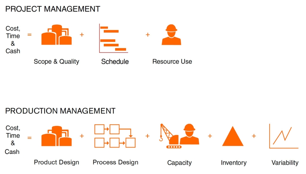
Figure 2: Comparing project management to Project Production Management
Operations Science then goes on to describe the relationship between the throughput of a flow, its cycle time (i.e., the time for the entity to traverse the flow), and its WIP via Little’s Law,
![]()
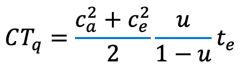
as well as the relationship between queue time, capacity utilization and variability in the Kingman approximation,
Operation Science also describes the components of cycle time, the meaning of “pull” and many other issues that are sometimes debated without end.
An immediate application to the preceding discussion is using Operations Science to describe how the Toyota Production System works.
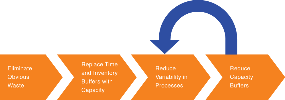
Figure 3: Implementing TPS
When there is variability in the process, OS principles show that there will always be either an accumulation of WIP between operations (if the WIP is not controlled directly) or a loss of output. A lot of WIP between processes makes for “efficient” production in terms of capacity utilization but is not efficient overall (long lead times, late delivery, poor quality, etc.). Toyota addresses this in the following way, as shown in Figure 2.
If Boeing had understood this, they probably would never have spent $250 million to install a moving assembly line for the 777 (which is no longer used for the 787, see Chapter 1 of Factory Physics for Managers, Pound, et al., 2104 for a complete discussion).
Though Ford and Ohno may have developed their approaches through constant tinkering and improvement, with invention of Operations Science, beginning in the early 1960’s, enabled by modern computer technologies, there exists no need to tinker. Production systems can and should be defined, designed and controlled (Hopp & Spearman, Factory Physics (Third Edition), 2011) (Hopp W. J., Supply Chain Science (First Edition), 2011) (Pound, Bell, & Spearman, Factory Physics for Managers: How Leaders Improve Performance in a Post-Lean Six-Sigma World, 2014) and elaborated upon for various forms of manufacturing and production.
The question we must address is how to achieve similar performance for an Oil and Gas Field Development project.
What does an Operations Science view of Onshore Field Development look like? Figure 4 gives a high-level view of operations encountered in onshore field development, which can be further broken down into individual activities and analyzed using the Operations Science laws, described earlier.

Figure 4: Onshore Field Development viewed as a Production System
In the beginning, drilling-related costs were the major element of field development investment, with drilling comprising over 60% of total well construction costs. In response, oil and gas producers opted for Frederick Taylor’s Scientific Management approach to managing field development where the goal is to maximize each operation’s individual efficiency in a production process.
As lateral drilling was integrated with hydraulic fracturing, the cost make-up of field development changed. For some, the cost of completion is more than drilling, with some surveys suggesting a 60% -40% split between completion and drilling as a proportion of total well cost. Much like automotive manufacture, the changing economics of field development has resulted in various strategies being deployed.
We remarked in the previous section that Ford and Ohno developed their approaches to manufacturing through constant tinkering and continuous improvement, but had they had an understanding of Operations Science, they could have developed optimum manufacturing approaches from OS principles considerably faster. We can make a similar remark for onshore field development – while different operators may be evolving their distinct approaches and drawing analogies with manufacturing, an OS perspective informs an optimum approach to onshore field development, such as described in (Nehring, Adopting Production Control: The Example of Onshore Field Development, 2017) (Nehring & Creech, Managing Variability, 2018) (Nehring, Onshore Field Development, 2016).
The OS approach to field development has been shown to have superior operational performance on certain metrics, as seen in a recent study by Wood Mackenzie (Wood Mackenzie, 2018). Figure 5 shows well costs achieved by different operators over 2012-2017, including Hess Corporation, which implemented Project Production Control for onshore field development in the Bakken, as described in (Nehring, Adopting Production Control: The Example of Onshore Field Development, 2017) (Nehring & Creech, Managing Variability, 2018) (Nehring, Onshore Field Development, 2016). As can be seen in Figure 5, the implementation of Project Production Control achieved steep reductions in well costs. Not shown in Figure 4 is that the variability of well costs achieved by Hess is lower than the variability of well costs achieved by others. In other words, Hess more consistently and repeatably achieved lower well costs since implementing OS in its field development than peers. Among the key changes, described in more detail in (Nehring & Creech, Managing Variability, 2018), was the steps they took to manage and reduce variability by the strategic choice of capacity buffers – in other words, consciously choosing not to maximize utilization of individual resources (like drilling rigs) and choosing not to use inventory as a buffer. This is quite a compelling argument for the efficacy of applying Operations Science and PPM in onshore field development.
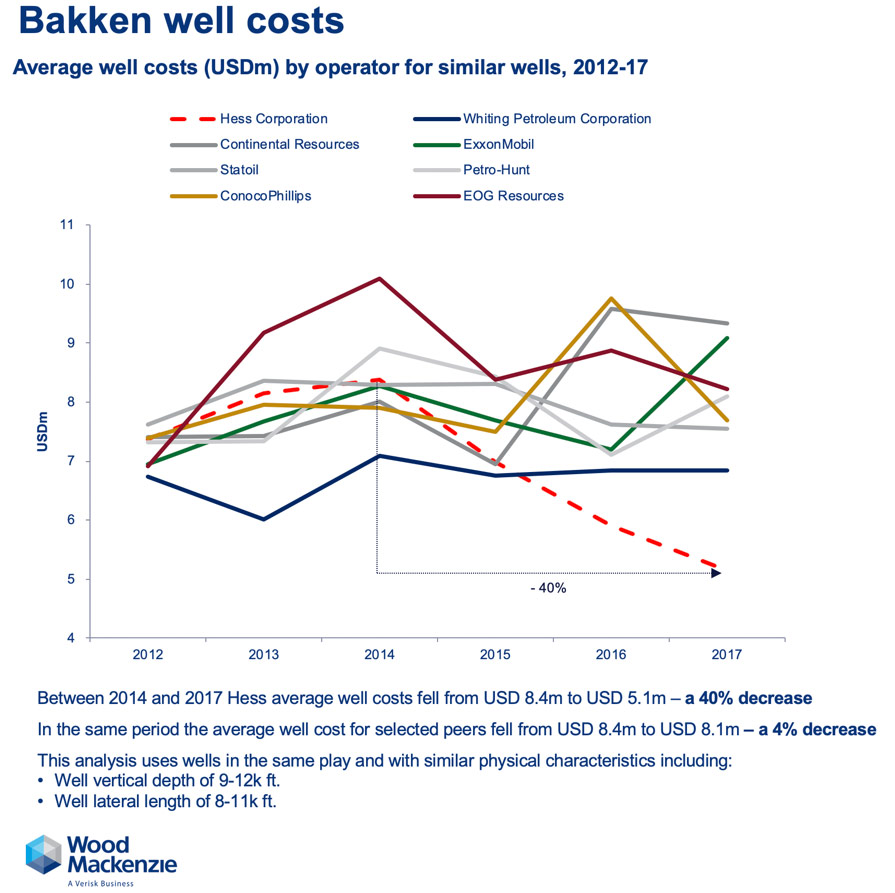
Figure 5: Comparing Bakken Well Costs for different operators 2012-2017
While many have drawn an analogy between recent approaches to onshore field development and manufacturing, we have made the case here that a more fundamental understanding of the science of production and operations is a more fruitful direction in order to identify effective ways to improve onshore field development. We reviewed the history of manufacturing approaches and showed that the technical framework of Operations Science leads to directly to optimized manufacturing. The Product-Process Matrix describes which types of production processes are suited to fabricating different products according to their degree of customization and volume. In particular, we highlighted that traditional manufacturing systems – like car assembly lines – are examples of production systems, but not all production systems are manufacturing systems. For example, onshore field development is a different type of production system, but nonetheless Operations Science provides the governing laws to optimize such systems. We cited (Nehring, Adopting Production Control: The Example of Onshore Field Development, 2017) (Nehring & Creech, Managing Variability, 2018) (Nehring, Onshore Field Development, 2016) which describe in detail the application of Operations Science in the form of Project Production Control (PPC) to onshore field development, and noted the benchmarking in (Wood Mackenzie, 2018) that demonstrated the superior operational performance achieved compared with peers. Some of the key conclusions are summarized below.
Oil and gas operators can accelerate their ability to reduce cost and free up cash through the effective application of Operations Science. Oil and gas operators should:
[1] A common but forgotten saying in the US in the early 1970s was “cheap stuff—made in Japan!”.
[2] The inventory buffer represents stock on-hand while the time buffer represents backorders. In service systems, there can be no stock, so all demand is essentially “backordered.”